5.4: The Magnetostatic Field Energy

Energy is required to establish a magnetic field. The energy density stored in a magnetostatic field established in a linear isotropic material is given by

\[\text{W}_{\text{B}}=\frac{\mu}{2} \text{H}^{2}=\frac{\vec{\text{H}} \cdot \vec{\text{B}}}{2} \quad \text { Joules } / \text{m}^{3}. \label{5.40}\]

The total energy stored in the magnetostatic field is obtained by integrating the energy density, W_B, over all space (the element of volume is d\(\tau\)):

\[\text{U}_{\text{B}}=\int \int \int_{S p a c e} \text{d} \tau\left(\frac{\vec{\text{H}} \cdot \vec{\text{B}}}{2}\right). \label{5.41}\]

This expression for the total energy, U_B, can be transformed into an integral over the sources of the magnetostatic field. The transformation can be carried out by means of the vector identity

\[\operatorname{div}(\vec{\text{A}} \times \vec{\text{H}})=\vec{\text{H}} \cdot(\vec{\nabla} \times \vec{\text{A}})-\vec{\text{A}} \cdot(\vec{\nabla} \times \vec{\text{H}}). \label{5.42}\]

(There is a nice discussion of this identity in The Feynman Lectures on Physics, Vol.II, section 27.3, by R.P.Feynman, R.B.Leighton, and M.Sands, Addison-Wesley, Reading, Mass.,1964). Proceed by integrating Equation (\ref{5.42}) over all space, then use Gauss’ theorem to transform the left hand side into a surface integral. The result is

\[\int \int_{S u r f a c e}(\vec{A} \times \vec{H}) \cdot d \vec{S}=\int \int \int_{V o l u m e} d \tau\left(\vec{H} \cdot \vec{B}-\vec{J}_{f} \cdot \vec{A}\right), \label{5.43}\]

where d\(\vec S\) is the element of surface area, \(\vec{\text{B}}=\vec{\nabla} \times \vec{\text{A}}=\operatorname{curl}(\vec{\text{A}})\), and \(\vec{\nabla} \times \vec{\text{H}}=\operatorname{curl}(\vec{\text{H}})=\vec{\text{J}}_{f}\). Here \(\vec A\) is the vector potential and \(\vec J_{f}\) is the current density. When the integrals in Equation (\ref{5.43}) are extended over all space the surface integral goes to zero: the surface area of a sphere of large radius R is proportional to R² but for currents confined to a finite region of space | \(\vec A\) | must decrease at least as fast as a dipole source, i.e. \(\propto 1 / \text{R}^{2}\), and | \(\vec H\) | must decrease at least as fast as 1/R³. It follows that in the large R limit the surface integral must go to zero like 1/R³. This requires the two terms on the right hand side of (\ref{5.43}) to be equal, and this result can be used to rewrite the expression (\ref{5.41}) in terms of the vector potential and the source current density:

\[\text{U}_{\text{B}}=\frac{1}{2} \int \int \int_{S p a c e} \text{d} \tau(\vec{\text{H}} \cdot \vec{\text{B}})=\frac{1}{2} \int \int \int_{S p a c e} \text{d} \tau\left(\vec{\text{J}}_{f} \cdot \vec{\text{A}}\right) . \label{5.44}\]

In many problems the current density is confined to a wire whose dimensions are small compared with other lengths in the problem. For such a circuit the contribution to the second volume integral in (\ref{5.44}) vanishes except for points within the wire, and therefore the volume integral can be replaced by a line integral along the wire providing that the variation of the vector potential, \(vec A\), over the cross-section of the wire can be neglected. For a wire of negligible thickness

\[\int \int \int_{Space} \text{d} \tau\left(\vec{\text{J}}_{f} \cdot \vec{\text{A}}\right) \rightarrow \text{I} \oint_{C} \vec{\text{A}} \cdot \text{d} \vec{\text{L}}, \label{5.45}\]

where I is the current through the wire; the current must be the same, of course, at all points along the circuit. The line integral of the vector potential around a closed circuit is equal to the magnetic flux, \(\Phi\), through the circuit. This equivalence can be seen by using the definition \(\vec B\) = curl(\(\vec A\)) along with Stokes’ theorem to transform the integral for the flux:

\[\Phi=\int \int_{S} \vec{\text{B}} \cdot \text{d} \vec{\text{S}}=\int \int_{S} \operatorname{curl}(\vec{\text{A}}) \cdot \text{d} \vec{\text{S}}=\oint_{C} \vec{\text{A}} \cdot \text{d} \vec{\text{L}} , \label{5.46}\]

where the curve C bounds the surface S. Combining Equations (\ref{5.46}) and (\ref{5.44}), the magnetic energy associated with a single circuit can be written

\[\text{U}_{\text{B}}=\frac{1}{2} \int \int \int_{S p a c e} \text{d} \tau\left(\vec{\text{J}}_{f} \cdot \vec{\text{A}}\right)=\frac{1}{2} \text{I} \Phi , \label{5.47}\]

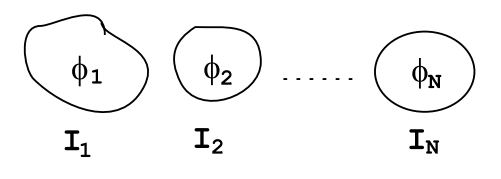
and for a number of circuits, N,

\[\text{U}_{\text{B}}=\frac{1}{2} \sum_{k=1}^{N} \text{I}_{\text{k}} \Phi_{k} . \label{5.48}\]

The latter expression is similar to Equation (3.3.6) for the electrostatic energy associated with a collection of charged conductors: currents in the magnetostatic case play a role similar to that of charges in the electrostatic case, and flux plays a role that is similar to the role played by the potentials.

Figure \(\PageIndex{7}\): N circuits embedded in a linear, isotropic medium. The magnetic fluxes, \(\Phi_{k}\), are linear functions of the currents I_j. The inductance coefficients satisfy the symmetry relations L_MN = L_NM.