5.3: A Discontinuity in the Permeability

Problems that involve currents embedded in materials for which the permeability varies from place to place are very difficult even if all of those materials exhibit linear response. Such problems can usually be solved by successive approximations: (1) the fields are calculated as if the source currents are immersed in a uniform permeable medium; (2) the resulting magnetization distribution is calculated from Equation (5.1.1) using the actual permeabilities; (3) the fields due to the effective current distribution \(\vec J\)_eff = curl(M) are added to the fields previously calculated; (4) the resulting total field is used to calculate a new magnetization distribution; (5) the cycle is repeated until adequate convergence has been secured, i.e. until the input field and the output field are essentially the same.

There is a class of magnetic problems that are very similar to electrostatic problems. In a region of space that is current free it is appropriate to use a magnetic scalar potential because curl(H) = 0. In any region in which the permeability does not depend upon position B = µH and therefore div(H) = 0 because div(B) = 0; in such a region the magnetic scalar potential, V_m, must satisfy LaPlace’s equation. The magnetic potential must also satisfy boundary conditions at a surface of discontinuity between regions which are characterized by different permeabilities. These boundary conditions are:

(1) V_m must be continuous across the interface between two materials. This condition is a consequence of curl(\(\vec H\)) = 0; the tangential components of \(\vec H\) must be continuous across the interface, as can be shown using Stokes’ theorem.

(2) The normal component of B must be continuous across the interface between two different materials. This condition is a consequence of div(\(\vec B\)) = 0; the continuity of the normal component of B can be deduced using Gauss’ theorem. In terms of the permeabilities one has

\[\mu_{1}\left(\frac{\partial \mathrm{V}_{\mathrm{m}}^{1}}{\partial \mathrm{n}}\right)_{\text {Boundary }}=\mu_{2}\left(\frac{\partial \mathrm{V}_{\mathrm{m}}^{2}}{\partial \mathrm{n}}\right)_{\text {Boundary }} , \label{5.22}\]

where \(\frac{\partial \mathrm{V}_{\mathrm{m}}}{\partial \mathrm{n}}\) is the derivative of the magnetic potential along the normal to the interface. These two boundary conditions are essentially the same as the boundary conditions imposed upon the electrostatic potential function. In addition, the magnetic potential must exhibit the proper behaviour at infinity and at the origin just like the electrostatic potential. The electrostatic potential and the magnetic potential both satisfy LaPlace’s equation, and both satisfy similar boundary conditions; it follows that similar problems must have correspondingly similar solutions. In particular, the magnetic potential functions for a sphere in a uniform applied field, and for a cylinder in a uniform field applied transverse to the cylinder axis must have the same form as those for the corresponding electrostatic problems discussed in Chpt.(3), sections(3.2.1 (c) and (d)) and Figures (3.2.4) and (3.2.5). For the magnetic case see Figures (5.3.2 and 5.3.3).

5.3.1 A Permeable Sphere in a Uniform Magnetic Field.

The potential function inside the sphere is given by

\[\mathrm{V}_{\mathrm{m}}^{\mathrm{i}}=-\frac{3\left(\frac{\mu_{2}}{\mu_{1}}\right) \mathrm{H}_{0}}{\left(1+2\left(\frac{\mu_{2}}{\mu_{1}}\right)\right)} \mathrm{r} \cos \theta . \label{5.23}\]

Figure \(\PageIndex{2}\): A permeable sphere placed in a uniform magnetic H-field of strength H₀ Amps/meter. The permeability of the sphere is µ₁, and it is placed in a medium having a permeability µ₂.

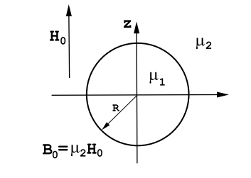
This corresponds to a uniform magnetic field along the z-axis. The potential function outside the sphere is given by

\[\mathrm{V}_{\mathrm{m}}^{\mathrm{o}}=-\mathrm{H}_{0} \mathrm{r} \cos \theta+\frac{\left(1-\left(\mu_{2} / \mu_{1}\right)\right)}{\left(1+2\left(\mu_{2} / \mu_{1}\right)\right)} \mathrm{R}^{3} \mathrm{H}_{0} \frac{\cos \theta}{\mathrm{r}^{2}} . \label{5.24}\]

This corresponds to a uniform magnetic field, H₀, plus the field of a point dipole located at the center of the sphere and having a strength

\[\mathrm{m}=\frac{\left(1-\left[\mu_{2} / \mu_{1}\right]\right)}{\left(1+2\left[\mu_{2} / \mu_{1}\right]\right)} 4 \pi \mathrm{R}^{3} \mathrm{H}_{0} \quad A m p-m^{2} . \nonumber \]

5.3.2 An Infinitely Long permeable Cylinder in a Uniform Magnetic Field.

The potential function inside the cylinder is given by

\[\mathrm{V}_{\mathrm{m}}^{\mathrm{i}}=-\frac{2\left(\mu_{2} / \mu_{1}\right) \mathrm{H}_{0}}{\left(1+\left(\mu_{2} / \mu_{1}\right)\right)} \mathrm{r} \cos \theta . \label{5.25}\]

Figure \(\PageIndex{3}\): An infinitely long permeable cylinder, radius R, placed in a uniform transverse magnetic field, H₀ Amps/meter. The axis of the cylinder is oriented along the z-axis. The permeability of the cylinder is µ₁ and the cylinder is immersed in a medium whose permeability is µ₂.

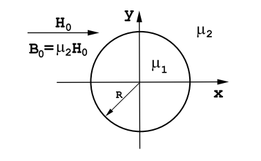
This corresponds to a uniform field along the x-axis, parallel with the applied magnetic field. The potential function outside the cylinder is given by

\[\mathrm{V}_{\mathrm{m}}^{\mathrm{o}}=-\mathrm{H}_{0} \mathrm{r} \cos \theta+\frac{\left(1-\left[\mu_{2} / \mu_{1}\right]\right)}{\left(1+\left[\mu_{2} / \mu_{1}\right]\right)} \mathrm{H}_{0} \mathrm{R}^{2} \frac{\cos \theta}{\mathrm{r}} . \label{5.26}\]

This corresponds to a uniform magnetic field, H₀, plus the field due to a line of dipoles located on the cylinder axis and having a strength

\[\mathrm{m}=2 \pi \mathrm{R}^{2} \mathrm{H}_{0} ; \frac{\left(1-\left[\mu_{2} / \mu_{1}\right]\right)}{\left(1+\left[\mu_{2} / \mu_{1}\right]\right)} \mathrm{H}_{0} \mathrm{R}^{2} \frac{\cos \theta}{\mathrm{r}} . \nonumber \]

5.3.3 A Point Magnetic Dipole Near a Permeable Plane.

There are no magnetic point charges, nevertheless the field of a point dipole can be considered to have its origin in two magnetic poles that are very close together. This suggests that the problem of a magnetic dipole near the plane interface between two magnetically dissimilar materials may be treated by the method of images by analogy with the corresponding electrostatic problem: see section(3.2.2(a) and (b)). The potential function for a magnetic point charge of strength q_m is given by

\[\text{V}_{\text{m}}=\frac{\text{q}_{\text{m}}}{4 \pi}\left(\frac{1}{\text{r}}\right) \nonumber \]

and the corresponding magnetic field, \(\vec H\), generated by a hypothetical point magnetic charge of strength q_m is given by the Coulomb law

\[\vec{\text{H}}=\frac{\text{q}_{\text{m}}}{4 \pi}\left(\frac{\vec{\text{r}}}{\text{r}^{3}}\right) . \label{5.27}\]

The corresponding field B is given by

\[ \vec{\text{B}}=\frac{\mu \text{q}_{\text{m}}}{4 \pi}\left(\frac{\vec{\text{r}}}{\text{r}^{3}}\right).\label{5.28}\]

Eqn.(\ref{5.27}) can be used to calculate the magnetic field generated by a magnetic dipole. Let a magnetic charge q_m be located at x=0, y=0, and z=d/2. Let a second magnetic charge -q_m be located at x=0, y=0, and z=- d/2. This pair of charges forms a magnetic dipole of strength m=qd oriented along the z-axis and positioned at z=0. The magnetic field of the dipole is given by (using Equation (\ref{5.27}))

\[\overrightarrow{\mathrm{H}}=\frac{\mathrm{q}_{\mathrm{m}}}{4 \pi} \frac{\left(\mathrm{x} \hat{\mathrm{u}}_{\mathrm{x}}+\mathrm{y} \hat{\mathrm{u}}_{\mathrm{y}}+(\mathrm{z}-\mathrm{d} / 2) \hat{\mathrm{u}}_{\mathrm{z}}\right)}{\left(\mathrm{x}^{2}+\mathrm{y}^{2}+(\mathrm{z}-\mathrm{d} / 2)^{2}\right)^{3 / 2}} - \frac{\mathrm{q}_{\mathrm{m}}}{4 \pi} \frac{\left(\mathrm{x} \hat{\mathrm{u}}_{\mathrm{x}}+\mathrm{y} \hat{\mathrm{u}}_{\mathrm{y}}+(\mathrm{z}+\mathrm{d} / 2) \hat{\mathrm{u}}_{\mathrm{z}}\right)}{\left(\mathrm{x}^{2}+\mathrm{y}^{2}+(\mathrm{z}+\mathrm{d} / 2)^{2}\right)^{3 / 2}}, \nonumber \]

or in the limit as d → 0 the expression for the magnetic field can be written

\[\vec{\text{H}}=\frac{1}{4 \pi}\left(\frac{3(\vec{\text{m}} \cdot \vec{\text{r}}) \vec{\text{r}}}{\text{r}^{5}}-\frac{\vec{\text{m}}}{\text{r}^{3}}\right) . \label{5.29}\]

Using \(\vec{\text{B}}=\mu \vec{\text{H}}\) this is the same result as stated in Equation (1.2.13) of Chpt.(1) for the case µ = µ₀.

The plane interface image problem for magnetic monopoles is shown in Figure (5.3.4). The H-field in the region on the left of the interface where the permeability is µ₁ is that due to the original magnetic charge q_m plus that due to an image charge of strength \(-\text{q}_{\text{m}}\left(\mu_{2}-\mu_{1}\right) /\left(\mu_{2}+\mu_{1}\right)\) located the

Figure \(\PageIndex{4}\): A fictitious magnetic point charge, qm, located outside the plane boundary between two permeable materials. The permeability to the left of the boundary is µ₁. The permeability on the right hand side of the boundary is µ₂. The magnetic charge is located a distance d from the interface. The other two magnetic charges, q_m′ and q_m” , are image charges.

Figure \(\PageIndex{5}\): Image problem for a magnetic dipole m0 located near the plane boundary between two permeable materials. The image dipole used for calculating fields on the left of the boundary is \(\text{m}_{0}^{\prime}=\text{m}_{0}\left(\frac{\mu_{2}-\mu_{1}}{\mu_{2}+\mu_{1}}\right)\). The image dipole used for calculating fields on the right of the plane boundary is \(\text{m}^{\prime \prime}=2 \text{m}_{0}\left(\frac{\mu_{1}}{\mu_{2}+\mu_{1}}\right)\). (N.B. the dipole strength is given by m₀ = q_md where d is the small separation between the plus and minus magnetic charges, NOT the distance d between the dipole and the interface at z=0.)

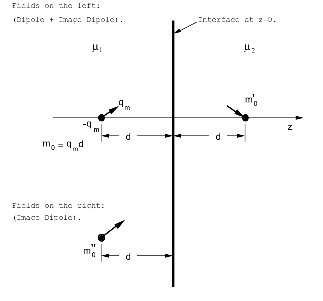
same distance behind the interface as q_m is located in front of the interface. The field in the right hand space, permeability µ₂, is the field due to a magnetic charge that is located at the same place as qm but whose strength is \(2 \text{q}_{\text{m}} \mu_{1} /\left(\mu_{2}+\mu_{1}\right)\). It is easy to show that the fields in the two regions are such that the components of H parallel with the interface are continuous across the interface. It is also easy to show that the normal components of H in the two regions is such that at the interface \(\mu_{1}(\vec{\text{H}})_{n}=\mu_{2}(\vec{\text{H}})_{n}\) so that the normal component of \(\vec B\) is continuous across the interface. Notice that the image charge is the negative of q_m for the case µ₂ > µ₁, but that the image charge has the same sign as qm when µ₂ < µ₁. The field on the left of the interface is given by

\[\vec{\text{H}}_{L}=\frac{\text{q}_{\text{m}}}{4 \pi}\left(\frac{\vec{\text{r}}_{1}}{\text{r}_{1}^{3}}\right)-\frac{\text{q}_{\text{m}}}{4 \pi}\left(\frac{\mu_{2}-\mu_{1}}{\mu_{2}+\mu_{1}}\right)\left(\frac{\vec{\text{r}}_{2}}{\text{r}_{2}^{3}}\right). \nonumber\]

The field on the right side of the interface is given by

\[\vec{\text{H}}_{R}=\frac{1}{4 \pi}\left(\frac{2 \text{q}_{\text{m}} \mu_{1}}{\mu_{2}+\mu_{1}}\right)\left(\frac{\vec{\text{r}}_{1}}{\text{r}_{1}^{3}}\right). \nonumber \]

This point charge solution can be extended by means of superposition to treat the problem of a magnetic dipole near a plane interface, Figure (5.3.5). The field on the left, in the region of permeability µ₁, is due to the dipole plus its image as shown in the figure. The fields in the region on the left due to the image dipole can be used to calculate the force and torque on the real dipole. The force on a magnetic monopole is given by

\[\vec{\text{F}}=\text{q}_{\text{m}} \vec{\text{B}}, \label{5.30}\]

The force on the magnetic dipole is just the sum of the forces acting on the two monopoles that make up the dipole: the dipole force is proportional to the field gradientr at the position of the dipole. The torque exerted on a magnetic dipole is given by

\[\vec{\text{T}}=\vec{\text{m}} \times \vec{\text{B}}. \label{5.31}\]

If µ₂ > µ₁ the magnetic dipole is attracted to the interface. Clearly this treatment can be generalized to discuss any permanently magnetized body located near a plane interface between two linear magnetic materials: the solution can be obtained as the superposition of the fields generated by the elementary dipoles of which the body is composed.

Figure \(\PageIndex{6}\): The image problem for the case of a line current of I Amps running parallel with the plane interface between two permeable materials and located a distance d from the interface.

5.3.4 A Wire Parallel with an Interface and carrying a Current of I Amps.

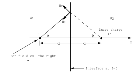
Another problem that can be solved using the method of images is that of a thin wire carrying a current, and oriented parallel with the plane interface between two different permeable regions as shown in Figure (5.3.6). The field in the region on the left is ascribed to the real current I plus an image current I’ located the same distance, d, to the right of the interface as the real current is located to the left of the interface. Any point P on the interface is equidistant from both the current I and its image, I’; let that distance be R. Let the line joining the position of the current to the point P on the interface make an angle \(\phi \) with the normal to the interface, as shown in Figure (5.3.6). The field lines generated by a long straight current carrying wire form concentric cylinders around the wire, and the strength of the field in free space is given by B_θ = µ₀I/2\(\pi\)R, where R is the distance from the wire; see Chpt.(4), Equation (4.3.3). This corresponds to an H-field H_θ = I/2\(\pi\)R Amps/m. The component of the magnetic field, \(\vec H\), parallel to the interface that is generated by the current I and its image I’ in Figure (5.3.6) is given by

\[\left.\mathrm{H}_{1}\right|_{\text {parallel}}=\frac{1}{2 \pi \mathrm{R}}\left(\mathrm{I} \cos \phi-\mathrm{I}^{\prime} \cos \phi\right). \label{5.32}\]

The field component normal to the interface is given by

\[\left.\mathrm{H}_{1}\right|_{\text {normal}}=\frac{1}{2 \pi \mathrm{R}}\left(\mathrm{I} \sin \phi+\mathrm{I}^{\prime} \sin \phi\right). \label{5.33}\]

Let the field in the region of space to the right of the interface be generated by an image current I” located at the position of the real current I. The magnetic field component parallel with the interface generated by I” is given by

\[\left.\mathrm{H}_{2}\right|_{\text {parallel}}=\frac{1}{2 \pi \mathrm{R}} \mathrm{I}^{"} \cos \phi, \label{5.34}\]

and its normal component is given by

\[\left.\mathrm{H}_{2}\right|_{\text {normal}}=\frac{1}{2 \pi \mathrm{R}} \mathrm{I}^{"} \sin \phi, \label{5.35}\]

The tangential component of H must be continuous across the interface, and therefore from Equations (\ref{5.32} and \ref{5.34})

\[\mathrm{I}-\mathrm{I}^{\prime}=\mathrm{I}^{"} . \label{5.36}\]

The normal component of \(\vec B\) must be continuous across the interface so that from Equations (\ref{5.33} and \ref{5.35}) one finds

\[\mu_{1}\left(\mathrm{I}+\mathrm{I}^{\prime}\right)=\mu_{2} \mathrm{I}^{\prime \prime} . \label{5.37}\]

The linear equations (\ref{5.36} and \ref{5.37}) can be solved to obtain the required image current strengths.The results are

\[\mathrm{I}^{\prime}=\left(\frac{\mu_{2}-\mu_{1}}{\mu_{2}+\mu_{1}}\right) \mathrm{I} , \label{5.38}\]

and

\[\mathrm{I}^{"}=\frac{2 \mathrm{I} \mu_{1}}{\left(\mu_{2}+\mu_{1}\right)} . \label{5.39}\]

The \(\vec H\) field in the space to the left of the interface is that generated by the current I plus the image current I’. The \(\vec H\) field to the right of the interface is that generated by the image current I”.