7.6: A Moving Point Charge in Vacuum

The charge density corresponding to a point charge is a singular distribution that can be written

\[\rho_{\text{f}}(\vec{\text{r}}, \text{t})=\text{q} \delta\left(\vec{\text{r}}-\vec{\text{r}}_{0}(\text{t})\right), \label{7.38}\]

where \(\delta(\vec{\text{r}}\)) is the Dirac delta-function introduced in Chapters (2) and (4), and \(\vec{\text{r}}_{0}(\text{t})\) describes the time variation of the position of the particle. The delta function is supposed to be zero for all values of its argument except when the argument is equal to zero; at that point the function becomes infinitely large but in such a manner that its integral is unity. The 1-dimensional \(\delta\)-function may be thought of as the limit as \(\epsilon\) → 0 of a very thin rectangular shape that is \(\epsilon\) wide and that has an amplitude 1/\(\epsilon\). The three dimensional \(\delta\)-function may be envisioned as the product of three 1-dimensional \(\delta\)-functions. The potential function that is generated by the distribution (\ref{7.38}) can be written using Equation (7.2.16):

\[\text{V}(\vec{\text{R}}, \text{t})=\frac{\text{q}}{4 \pi \epsilon_{0}} \int \int \int_{S p a c e} \text{d} \tau \frac{\delta\left[\vec{\text{r}}-\vec{\text{r}}_{0}\left(\text{t}_{\text{R}}\right)\right]}{|\vec{\text{R}}-\vec{\text{r}}|}. \label{7.39}\]

The integrand is very sharply peaked when \(\vec{\text{r}}=\vec{\text{r}}_{0}\left(\text{t}_{\text{R}}\right)\) so that it is very tempting to conclude that

\[\text{V}(\vec{\text{R}}, \text{t})=\frac{\text{q}}{4 \pi \epsilon_{0}} \frac{1}{\left|\vec{\text{R}}-\vec{\text{r}}_{0}\left(\text{t}_{\text{R}}\right)\right|}. \nonumber \]

This equation is WRONG, because it ignores the position dependence of the retarded time which appears in the argument of the \(\delta\)−function. In

Figure \(\PageIndex{i}\): A small blob of charge moving along the x-axis with a velocity vx. The contribution to the potential at P at the time of observation, t, comes from the position of the particle at the retarded time t_R = t − r₀/c.

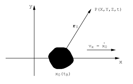
order to understand this, suppose for simplicity that a co-ordinate system is chosen so that at the retarded time the particle is moving along the x-axis, i.e. y₀ = z₀ = 0 and y,z are not changing with time because the velocity of the particle is directed along x (see Figure (7.6.4)). The integral of Equation (\ref{7.39}) can be written explicitly in cartesian co-ordinates: the result is

\[\text{V}(\text{X}, \text{Y}, \text{Z}, \text{t})=\frac{\text{q}}{4 \pi \epsilon_{0}} \int \int \int_{-\infty}^{+\infty} \text{d} \text{xdydz} \frac{\delta\left[\text{x}-\text{x}_{0}\left(\text{t}_{\text{R}}\right)\right] \delta[\text{y}] \delta[\text{z}]}{\sqrt{(\text{X}-\text{x})^{2}+(\text{Y}-\text{y})^{2}+(\text{Z}-\text{z})^{2}}}. \nonumber\]

The integrations over y,z are just ordinary integrations over \(\delta\)−functions that may be carried out at once using

\[\int_{-\infty}^{+\infty} \operatorname{du} \text{f}(\text{u}) \delta(\text{u})=\text{f}(0). \nonumber \]

This leaves the integration over x to be carried out;

\[\text{V}(\text{X}, \text{Y}, \text{Z}, \text{t})=\frac{\text{q}}{4 \pi \epsilon_{0}} \int_{-\infty}^{+\infty} \text{d} \text{x} \frac{\delta\left[\text{x}-\text{x}_{0}\left(\text{t}_{\text{R}}\right)\right]}{\sqrt{(\text{X}-\text{x})^{2}+\text{Y}^{2}+\text{Z}^{2}}}. \label{7.40}\]

In order to turn (\ref{7.40}) into an ordinary integration over a \(\delta\)−function it is necessary to change variables so as to get rid of the spatial variation that is contained in the retarded time, t_R. Introduce the new variable

\[\text{u}=\text{x}-\text{x}_{0}\left(\text{t}_{\text{R}}\right). \nonumber \]

Then

\[\text{du}=\text{dx}-\dot{\text{x}}_{0}\left(\frac{\partial \text{t}_{\text{R}}}{\partial \text{x}}\right) \text{dx}, \nonumber \]

where

\[\text{t}_{\text{R}}=t-\frac{\sqrt{(\text{X}-\text{x})^{2}+\text{Y}^{2}+\text{Z}^{2}}}{\text{c}}, \nonumber \]

so that

\[\frac{\partial \text{t}_{\text{R}}}{\partial \text{x}}=\frac{(\text{X}-\text{x})}{\text{c} \sqrt{(\text{X}-\text{x})^{2}+\text{Y}^{2}+\text{Z}^{2}}}. \nonumber \]

One finally obtains for the differential du the expression

\[\text{du}=\text{dx}\left(1-\frac{\dot{\text{x}}_{0}(\text{X}-\text{x})}{\text{c} \sqrt{(\text{X}-\text{x})^{2}+\text{Y}^{2}+\text{Z}^{2}}}\right), \nonumber \]

and the integral (\ref{7.40}) becomes

\[\text{V}(\text{X}, \text{Y}, \text{Z}, \text{t})=\frac{\text{q}}{4 \pi \epsilon_{0}} \int_{-\infty}^{+\infty} \text{du} \frac{\delta(\text{u})}{\left(\sqrt{(\text{X}-\text{x})^{2}+\text{Y}^{2}+\text{Z}^{2}}-\frac{\dot{x_{0}}(\text{x}-\text{x})}{\text{c}}\right)}. \nonumber \]

The expression for the potential function has been transformed into a \(\delta\)−function integration that can be carried out immediately to give

\[\text{V}(\text{X}, \text{Y}, \text{Z}, \text{t})=\frac{\text{q}}{4 \pi \epsilon_{0}}\left(\frac{1}{\sqrt{\left(\text{X}-\text{x}_{0}\right)^{2}+\text{Y}^{2}+\text{Z}^{2}}-\frac{\dot{x_{0}}\left(\text{X}-\text{x}_{0}\right)}{\text{c}}}\right)_{\text{t}_{\text{R}}}, \label{7.41} \]

since for u=0 x=x₀(t_R). The result, Equation (\ref{7.41}), can be written in a more general and compact form using vector notation:

\[\text{V}(\vec{\text{R}}, t)=\frac{\text{q}}{4 \pi \epsilon_{0}}\left(\frac{1}{\left|\vec{\text{r}}_{0}\right|-\frac{\vec{v} \cdot \vec{r}_{0}}{c}}\right)_{t-r_{0} / \text{c}} , \label{7.42}\]

where \(\vec{\text{r}}_{0}=(\vec{\text{R}}-\vec{\text{r}})\) is the vector that specifies the position of the particle at the retarded time relative to the point of observation at time t, P(X,Y,Z,t) (see Figure (7.4)), and \(\vec v\) is the particle velocity at the retarded time.

Feynman (loc.cit. section 21-5) has given a very physical description of why the retarded potential contains the complicated denominator of Equation (\ref{7.42}) rather than simply the retarded distance | r₀ |. He explains how the volume integration of (\ref{7.39}) for the potential must explicitly take into account that the contribution to the potential at a fixed time of observation comes from different retarded times for different points in the charge distribution.

Exactly the same arguments apply to the calculation of the vector potential for a moving point charge from Equation (7.2.18). The current density for a point charge moving with a velocity \(\vec v\) is given by

\[\vec{\text{J}}(\vec{\text{r}}, t)=\text{q} \vec{\text{v}} \delta\left(\vec{\text{r}}-\vec{\text{r}}_{0}(\text{t})\right), \nonumber \]

where \(\vec{\text{r}}_{0}(\text{t})\) describes the position of the particle at time t. Upon carrying out the integration in Equation (7.2.18) the resulting vector potential is found to be

\[\vec{\text{A}}(\vec{\text{R}}, \text{t})=\frac{\mu_{0}}{4 \pi}\left(\frac{\text{q} \vec{\text{v}}}{\left|\vec{\text{r}}_{0}\right|-\frac{\vec{v} \cdot \vec{r}_{0}}{\text{c}}}\right)_{\text{t}-\text{r}_{0} / \text{c}}, \label{7.43}\]

where \(\vec{\text{r}}_{0}\) is the vector drawn from the position of the particle at the retarded time, t_R, to the point of observation at time t. Eqns.(\ref{7.42}) and (\ref{7.43}) are called the Lienard-Wiechert potentials for a point charge. They are consistent with the theory of relativity. The electric and magnetic fields generated by a moving point charge, Chpt.(1), Equations (1.1.9) and (1.1.10), can be deduced from them by means of the relations

\[\vec{\text{B}}=\operatorname{curl}(\vec{\text{A}}), \nonumber\]

and

\[\vec{\text{E}}=-\vec{\operatorname{grad}}(\text{V})-\frac{\partial \vec{\text{A}}}{\partial \text{t}} . \nonumber\]

In the general case these result in the rather complex equations of Equations (1.1.9) and (1.1.10). However, in the limit v/c ≪ 1 the fields generated by a moving point charge can be obtained relatively simply from the low velocity limit of the vector potential. Consider a charge q near the origin, at \(\vec{\text{r}}=(0,0, \xi)\), and moving along the z-axis with a velocity \(v=\dot{\xi}\). In spherical polar co-ordinates one has

\[\begin{aligned}
\text{A}_{\text{r}}=& \frac{\mu_{0}}{4 \pi} \frac{\text{qv} \cos \theta}{\left(\text{r}-\frac{\text{v} \text{z}}{\text{c}}\right)}=\frac{\mu_{0}}{4 \pi} \frac{\text{qv} \cos \theta}{\text{r}\left(1-\frac{\text{v} \cos \theta}{\text{c}}\right)} \\
\text{A}_{\theta} &=-\frac{\mu_{0}}{4 \pi} \frac{\text{qv} \sin \theta}{\text{r}\left(1-\frac{\text{v} \cos \theta}{\text{c}}\right)}.
\end{aligned}\]

For a slowly moving particle, v ≪ c, these become

\[\text{A}_{\text{r}}=\frac{\mu_{0}}{4 \pi} \frac{\text{qv} \cos \theta}{\text{r}}, \nonumber \]

and

\[\text{A}_{\theta}=-\frac{\mu_{0}}{4 \pi} \frac{\text{qv} \sin \theta}{\text{r}}, \nonumber \]

where \(\text{A}_{\phi}=0\), \(\text{v}=\dot{\xi}\), and A_r , A_θ are to be evaluated at the retarded time t_R = t − r/c. The magnetic field is given by \(\vec{\text{B}}=\operatorname{curl}(\vec{\text{A}})\):

\[\text{B}_{\text{r}}=\text{B}_{\theta}=0, \nonumber \]

and

\[\text{B}_{\phi}=\frac{1}{\text{r}} \frac{\partial}{\partial \text{r}}\left(\text{rA}_{\theta}\right)-\frac{1}{\text{r}} \frac{\partial}{\partial \theta}\left(\text{A}_{\text{r}}\right), \nonumber \]

where \(\frac{\partial}{\partial \text{r}}\) includes a term −∂/c∂t because if r changes by dr the retarded time changes by dt_R = −dr/c. Thus

\[\text{B}_{\phi}=\frac{\mu_{0}}{4 \pi} \text{q} \sin \theta\left[\frac{\text{v}}{\text{r}^{2}}+\frac{\dot{\text{v}}}{\text{cr}}\right]. \label{7.44}\]

Eqn.(\ref{7.44}) is just the field generated by a point electric dipole at the origin if one writes \(\text{p}_{\text{z}}=\text{q} \xi\), \(\dot{\text{p}}_{\text{z}}=\text{q} \dot{\xi}\), and \(\ddot{\text{p}}_{z}=\text{q} \ddot{\xi}\); then

\[\text{B}_{\phi}=\frac{\mu_{0}}{4 \pi} \sin \theta\left[\frac{\dot{\text{p}_{\text{z}}}}{\text{r}^{2}}+\frac{\ddot{\text{p}}_{\text{z}}}{\text{cr}}\right], \label{7.45}\]

see Equation (7.4.2).

The electric field can be calculated from

\[\operatorname{curl}(\vec{\text{B}})=\frac{1}{\text{c}^{2}} \frac{\partial \vec{\text{E}}}{\partial \text{t}}. \nonumber \]

Thus

\[\frac{1}{c^{2}} \frac{\partial \text{E}_{\text{r}}}{\partial \text{t}}=\frac{\mu_{0}}{4 \pi} 2 \cos \theta\left[\frac{\text{qv}}{\text{r}^{3}}+\frac{\dot{\text{v}}}{\text{cr}^{2}}\right], \nonumber \]

or

\[\frac{\partial \text{E}_{\text{r}}}{\partial \text{t}}=\frac{1}{4 \pi \epsilon_{0}} 2 \cos \theta\left[\frac{\dot{\text{p}_{\text{z}}}}{\text{r}^{3}}+\frac{\ddot{\text{p}}_{\text{z}}}{\text{cr}^{2}}\right]. \nonumber \]

This last equation can be integrated with respect to the time to obtain

\[\text{E}_{\text{r}}=\text{E}_{0}+\frac{2 \cos \theta}{4 \pi \epsilon_{0}}\left[\frac{\text{p}_{\text{z}}}{\text{r}^{3}}+\frac{\dot{\text{p}}_{\text{z}}}{\text{cr}^{2}}\right], \label{7.46}\]

where the constant of integration is simply the static field due to a charge, q, at the origin,

\[\text{E}_{0}=\frac{1}{4 \pi \epsilon_{0}} \frac{\text{q}}{\text{r}^{2}}. \nonumber \]

The radial electric field component is that of a point charge at the origin plus a field due to a point dipole at the origin.

The transverse electric field component is given by

\[\frac{\partial \text{E}_{\theta}}{\partial \text{t}}=\frac{\sin \theta}{4 \pi \epsilon_{0}}\left[\frac{\dot{\text{p}}_{z}}{\text{r}^{3}}+\frac{\ddot{\text{p}}_{z}}{\text{cr}^{2}}+\frac{\dddot{\text{p}}_{z}}{\text{c}^{2} \text{r}}\right]. \nonumber \]

This expression can be integrated to give

\[\text{E}_{\theta}=\frac{\sin \theta}{4 \pi \epsilon_{0}}\left[\frac{\text{p}_{\text{z}}}{\text{r}^{3}}+\frac{\dot{\text{p}}_{\text{z}}}{\text{cr}^{2}}+\frac{\ddot{\text{p}}_{\text{z}}}{\text{c}^{2} \text{r}}\right]. \label{7.47}\]

For this case the constant of integration is zero because in the static limit the only contribution to the θ-component of the electric field is a dipole term due to the displacement of the charge from the origin by the vanishingly small distance ξ. Eqn.(\ref{7.47}) is just the θ-component of the field generated by a point electric dipole at the origin, Equation (7.4.3). The radiation field terms, the terms that fall off like 1/r, can be written

\[\text{E}_{\theta}=\frac{\sin \theta}{4 \pi \epsilon_{0}} \frac{\text{qa}}{\text{c}^{2} \text{r}}, \nonumber \]

\[\text{cB}_{\phi}=\frac{\sin \theta}{4 \pi \epsilon_{0}} \frac{\text{qa}}{\text{c}^{2} \text{r}}, \nonumber \]

where \(a=\ddot{\xi}\). These radiation fields can be written as follows in terms of general vector position co-ordinates where the particle is taken to be at the origin:

\[\vec{\text{E}}(\vec{\text{r}}, \text{t})=\left.\frac{\text{q}}{4 \pi \epsilon_{0}} \frac{[\vec{\text{r}} \times \vec{\text{r}} \times \vec{\text{a}}]}{\text{c}^{2} \text{r}^{3}}\right|_{\text{t}_{\text{R}}}\label{7.48}\]

\[\text{c} \vec{\text{B}}(\vec{\text{r}}, \text{t})=\left.\frac{\text{q}}{4 \pi \epsilon_{0}} \frac{|\vec{\text{a}} \times \vec{\text{r}}|}{\text{c}^{2} \text{r}^{2}}\right|_{\text{t}_{\text{R}}}, \nonumber \]

where the acceleration \(\vec a\) is evaluated at the retarded time t_R = t − r/c.

Eqns.(\ref{7.48}) are valid only for a slowly moving charge whose velocity is very much smaller than the velocity of light in vacuum. These radiation fields fall off as the first power of the distance from the observer to the particle.

Eqns.(\ref{7.46} and \ref{7.47}) can also be calculated from the formula

\[\vec{\text{E}}=-\vec{\operatorname{grad}}(\text{V})-\frac{\partial \vec{\text{A}}}{\partial \text{t}}, \nonumber \]

using the low velocity limit for the vector potential along with the expression for the potential function, Equation (\ref{7.42}), expanded to lowest order in the small quantities ξ and \(\dot{\xi} / \text{c}\):

\[\text{V}(\vec{\text{r}}, \text{t})=\frac{\text{q}}{4 \pi \epsilon_{0}} \frac{1}{\text{r}}\left[1+\frac{\xi \cos \theta}{\text{r}}+\frac{\dot{\xi} \cos \theta}{\text{c}}\right]. \nonumber \]