7.4: An Electric Dipole Radiator

An atom or a molecule in an excited state may develop an oscillating electric dipole moment density, \(\vec P\). This dipole density oscillates at a frequency that ~ is proportional to the energy difference between the excited state and the ground state, \(\Delta \text{E}: \hbar \omega=\Delta \text{E}\). The oscillating dipole moment generates an electromagnetic field that carries off the excited state energy ∆E, and the atom or molecule returns to the ground state. An oscillating dipole moment density constitutes a current density. From Equation (7.2.3)

\[\vec{\text{J}}_{T}=\frac{\partial \vec{\text{P}}}{\partial \text{t}}=\vec{\text{P}}, \nonumber \]

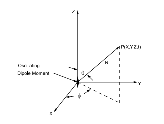
if \(\vec{\text{J}}_{f}\) and \(\vec M\) are both zero as shall be assumed here. Also assume that the ~ dipole density has only a z-component as shown in Figure (7.4.3). Then from

Figure \(\PageIndex{3}\): The co-ordinate system used to describe the fields generated by an oscillating atomic or molecular electric dipole moment.

Equation (7.2.18) the vector potential can be written

\[\text{A}(\vec{\text{R}}, t)=\frac{\mu_{0}}{4 \pi} \frac{1}{\text{R}} \int \int \int_{V o l} \text{d} \tau \dot{\text{P}}_{\text{z}}(\vec{\text{r}}, t-\text{R} / \text{c}) , \nonumber \]

where d\(\tau\) is the element of volume and the integral is carried out over the volume, Vol, of the atom or molecule. In the above equation it has been assumed that the dimensions of the atom or molecule are so small that all parts are at the same distance from the observer: ie. as \(\vec r\) in (7.2.18) ranges over the volume, Vol, changes in the distance to the observer can be neglected both in the denominator and in the retarded time. This is the point dipole approximation. The volume integration with this assumption simply gives the total atomic or molecular dipole moment, \(\vec{\text{p}}_{\text{z}}\), and

\[\text{A}_{\text{z}}(\text{R}, \theta, \phi, t)=\frac{\mu_{0}}{4 \pi} \frac{\dot{\text{p}}_{\text{z}}}{\text{R}} , \nonumber \]

where \(\dot{\text{p}}_{\text{z}}\) is the total dipole moment evaluated at the retarded time t_R = t − R/c . This vector potential can now be used to calculate the magnetic field, \(\vec{\text{B}}=\operatorname{curl}(\vec{\text{A}})\). For this purpose it is convenient to use spherical polar co-ordinates, see Figure (7.4.3):

\[\text{A}_{\text{R}}(\text{R}, \theta, \text{t})=\frac{\mu_{0}}{4 \pi} \frac{\dot{\text{p}}_{\text{z}}(\text{t}-\text{R} / \text{c})}{\text{R}} \cos \theta , \label{7.29}\]

\[\begin{aligned}
&\text{A}_{\theta}(\text{R}, \theta, \text{t})=-\frac{\mu_{0}}{4 \pi} \frac{\dot{\text{p}}_{\text{z}}(\text{t}-\text{R} / \text{c})}{\text{R}} \sin \theta,\\
&\text{A}_{\phi}(\text{R}, \theta, \text{t})=0. \nonumber
\end{aligned}\]

Notice that the vector potential does not depend on the angle \(\phi\) so that the operator (∂/∂\(\phi\)) gives zero. From (\ref{7.29}) one finds

\[\text{B}_{\text{R}}=\text{B}_{\theta}=0 , \nonumber \]

and

\[\text{B}_{\phi}=\frac{1}{\text{R}}\left[\frac{\partial}{\partial \text{R}}\left(\text{R} \text{A}_{\theta}\right)-\frac{\partial \text{A}_{\text{R}}}{\partial \theta}\right] , \nonumber \]

or

\[\text{B}_{\phi}=\frac{\mu_{0}}{4 \pi}\left[\frac{\ddot{\text{p}}_{\text{z}}}{\text{cR}}+\frac{\dot{\text{p}}_{\text{z}}}{\text{R}^{2}}\right] \sin \theta. \label{7.30}\]

(Remember that \(\partial \dot{\text{p}}_{z} / \partial \text{R}=-\ddot{\text{p}}_{z} / \text{c}\) because the dipole moment must be evaluated at the retarded time, t_R = t−R/c). The electric field components can be most easily calculated from the maxwell equation \(\operatorname{curl}(\vec{\text{B}})=\left(1 / \text{c}^{2}\right) \partial \vec{\text{E}} / \partial \text{t}\) since outside the atom or molecule \(\vec{\text{J}}_{T}=0\). The components of \(\operatorname{curl}(\vec{\text{B}})\) are:

\[\operatorname{curl}(\vec{\text{B}})_{\text{R}}=\frac{1}{\text{R} \sin \theta} \frac{\partial}{\partial \theta}\left(\sin \theta \text{B}_{\phi}\right) , \nonumber\]

so that

\[\begin{array}{c}
\operatorname{curl}(\vec{\text{B}})_{\text{R}}=\frac{\mu_{0}}{4 \pi}\left[\frac{\ddot{\text{p}}_{\text{z}}}{\text{cR}^{2}}+\frac{\dot{\text{p}}_{\text{z}}}{\text{R}^{3}}\right] \cos \theta \\
\operatorname{curl}(\vec{\text{B}})_{\theta}=-\frac{1}{\text{R}} \frac{\partial}{\partial \text{R}}\left(\text{RB}_{\phi}\right) \nonumber
\end{array} \]

so that

\[\operatorname{curl}(\vec{\text{B}})_{\theta}=\frac{\mu_{0}}{4 \pi}\left(\frac{\ddot{\text{p}}_{\text{z}}}{\text{c}^{2} \text{R}}+\frac{\ddot{\text{p}}_{\text{z}}}{\text{c} \text{R}^{2}}+\frac{\dot{\text{p}}_{\text{z}}}{\text{R}^{3}}\right) \sin \theta. \]

Finally,

\[\operatorname{curl}(\vec{\text{B}})_{\phi}=0. \nonumber \]

The electric field components are therefore given by

\[\text{E}_{\text{R}}=\frac{1}{2 \pi \epsilon_{0}}\left[\frac{\dot{\text{p}}_{\text{z}}}{\text{cR}^{2}}+\frac{\text{p}_{\text{z}}}{\text{R}^{3}}\right] \cos \theta, \label{7.31}\]

\[\text{E}_{\theta}=\frac{1}{4 \pi \epsilon_{0}}\left[\frac{\ddot{\text{p}}_{z}}{\text{c}^{2} \text{R}}+\frac{\dot{\text{p}}_{z}}{\text{cR}^{2}}+\frac{\text{p}_{z}}{\text{R}^{3}}\right] \sin \theta, \nonumber\]

\[\text{E}_{\phi}=0. \nonumber \]

The electric field derivatives from \(\operatorname{curl}(\vec{\text{B}})\) have been integrated with respect to time, and \(c^{2}=1 /\left(\mu_{0} \epsilon_{0}\right)\) has been used to eliminate µ₀.

The fields generated by a point dipole fall naturally into two groups:

(a) The Near Fields. These are the terms that become dominant as R, the distance from dipole to observer, becomes small. They are

\[\text{B}_{\phi}=\frac{\mu_{0}}{4 \pi} \frac{\dot{\text{p}}_{z}}{\text{R}^{2}} \sin \theta, \label{7.32}\]

\[\text{E}_{\text{R}}=\frac{1}{4 \pi \epsilon_{0}} \frac{2 \text{p}_{\text{z}} \cos \theta}{\text{R}^{3}}, \nonumber\]

\[\text{E}_{\theta}=\frac{1}{4 \pi \epsilon_{0}} \frac{\text{p}_{z} \sin \theta}{\text{R}^{3}}. \nonumber \]

The magnetic field is just that generated by a static current element according to the law of Biot-Savart, see Equation (4.2.2). The electric field components have the same form as those generated by a static dipole oriented along the z-axis, see Equation (1.2.12). Therefore near the dipole retardation effects are unimportant as one would expect.

(b) The Far Fields or the Radiation Fields. Far from the dipole the dominant terms for both the electric and magnetic fields are those that fall off with distance like 1/R.

\[\text{B}_{\phi}=\frac{\mu_{0}}{4 \pi} \frac{\ddot{\text{p}}_{\text{z}}}{\text{cR}} \sin \theta, \label{7.33}\]

\[\begin{aligned}
\text{E}_{\text{R}} & \rightarrow 0 \quad \operatorname{like}\left(1 / \text{R}^{2}\right) \\
\text{E}_{\theta} &=\frac{\mu_{0}}{4 \pi} \frac{\ddot{\text{p}}_{\text{z}}}{\text{R}} \sin \theta \\
&=\frac{1}{4 \pi \epsilon_{0}} \frac{\ddot{\text{p}}_{\text{z}}}{\text{c}^{2} \text{R}} \sin \theta
\end{aligned}\]

In this limit E_θ = cB_\(\phi\), and the electric and magnetic fields are orthogonal. Moreover, both the electric and magnetic field are orthogonal to the line joining the observer to the dipole. These radiation fields are said to be transverse fields. Note particularly that the dipole moment is to be calculated at the retarded time, t_R = t − R/c, where t is the time of observation. Any fields created by the dipole at a particular instant require a transit time R/c to reach the observer.