8.5: Scattering from a Stationary Atom

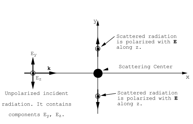
Let plane wave radiation propagating in vacuum fall upon a stationary atom located at the origin of co-ordinates. Let the plane wave be polarized with the electric vector directed along \(z\), and let the wave be propagating along \(x\) (Figure (8.4.5)):

\[\mathrm{E}_{\mathrm{z}}=\mathrm{E}_{0} \exp i(\mathrm{kx}-\omega \mathrm{t}). \label{8.25}\]

We will consider only radiation whose wavelength, λ, is much larger than the dimensions of the atom, i.e. much larger than 10⁻¹⁰ meters. This condition restricts the frequency of the radiation to f ≤ 3×10¹⁷ Hz. In this long wavelength limit one can take the electric field to be uniform over the atom. Each charged particle in the atom will be subjected, as a first approximation, to the electric field of Equation (\ref{8.25}). The response of the nucleus to the oscillating electric field can be neglected for purposes of estimating the induced atomic electric dipole moment because the nucleus is so massive compared with the electrons. The main contribution to the induced dipole moment will be due to the response of the cloud of electrons to the applied oscillating electric field. The results of calculations using quantum mechanics shows that the electrons behave like simple harmonic oscillators that follow an equation of motion of the form

\[\frac{\mathrm{d}^{2} \mathrm{z}}{\mathrm{dt}^{2}}+\omega_{0}^{2} \mathrm{z}=-\frac{|\mathrm{e}|}{\mathrm{m}} \mathrm{E}_{0} \mathrm{e}^{-i \omega t} , \label{8.26}\]

where \(\omega_{0}^{2}\) is the square of the natural frequency associated with the electron. (Quantum mechanics must be used to calculate the resonant frequencies associated with the various electron groups in an atom). The steady state solution of Equation (\ref{8.26}) is

\[\mathrm{z}(\mathrm{t})=\mathrm{z}_{0} \mathrm{e}^{-i \omega t}, \label{8.27}\]

where

\[\mathrm{z}_{0}=\frac{\left(\frac{|\mathrm{e}|}{\mathrm{m}}\right) \mathrm{E}_{0}}{\left(\omega^{2}-\omega_{0}^{2}\right)}. \label{8.28}\]

In Equation (\ref{8.28}) | e |= 1.602 × 10⁻¹⁹ Coulombs, the electron charge, and m=9.11 × 10⁻³¹ kg, the electron mass. The electron develops an oscillating dipole moment, p_z = − | e | z, as a result of the motion induced by the forcing electric field. The oscillating dipole will radiate energy at the same frequency as the incident radiation, and in this way energy will be removed from the incident plane wave and scattered in all directions around the z-axis as per the discussion of section (8.2), Equation (8.2.10). If the atom contains many groups of electrons, each group characterized by a characteristic resonant frequency, ωn, then each group will develop a dipole moment as a result of a vibration of the form of Equation (\ref{8.27}). The total dipole moment developed by the atom is obtained by summing the contributions from each electron group:

\[\mathrm{p}_{\mathrm{z}}=-\left(\frac{\mathrm{e}^{2}}{\mathrm{m}}\right)\left(\sum_{\mathrm{n}} \frac{\mathrm{f}_{\mathrm{n}}}{\left(\omega^{2}-\omega_{0}^{2}\right)}\right) \mathrm{E}_{0} \mathrm{e}^{-i \omega \mathrm{t}}=\mathrm{p}_{0} \mathrm{e}^{-i \omega \mathrm{t}}. \label{8.29}\]

The factors f_n are called the oscillator strengths. Each f_n is a measure of the effective number of electrons in a particular group characterized by the resonant frequency ω_n. The above model does not include damping processes and therefore the response described by Equation (\ref{8.29}) becomes infinite whenever the frequency of the incident radiation becomes equal to one of the resonant frequencies, ω_n. In any actual atomic system the response of the electrons is limited by a number of energy loss mechanisms, including the energy radiated by the oscillating dipole moment, so that at resonance the electronic response becomes large but it does remain finite. The rate at which energy is scattered into the direction specified by θ,φ is given by Equation (8.2.10) of section (8.2) :

\[<\mathrm{S}_{\mathrm{r}}>=\frac{1}{8 \pi} \frac{\mathrm{c}}{4 \pi \epsilon_{0}}\left(\frac{\omega}{\mathrm{c}}\right)^{4} \frac{\mathrm{p}_{0}^{2} \sin ^{2} \theta}{\mathrm{R}^{2}}, \label{8.30}\]

where p₀ is given by Equation (\ref{8.29}). A number of interesting conclusions can be drawn from the above result:

1. No energy is scattered along the direction parallel with the incident electric field;
2. The intensity of the scattered radiation is maximum in the plane perpendicular to the direction of the incident light electric vector, and the scattered light will be linearly polarized;
3. For frequencies that are much less than the lowest atomic resonant frequency the dipole moment, Equation (\ref{8.29}), becomes independent of frequency. Under these conditions the intensity of the scattered radiation increases very rapidly with frequency; it is proportional to ω⁴ ;
4. In the high frequency limit, ω ≫ ω_max, where ω_max is the greatest resonant frequency, the dipole moment amplitude becomes inversely proportional to the square of the frequency so that the intensity of the scattered radiation becomes independent of frequency.

If one observes the result of scattering of visible, unpolarized light from atoms or molecules in a direction that is perpendicular to the direction of propagation of the incident light, it will be found that the scattered light will tend to be blue and it will be linearly polarized, see Figure (8.5.6). The scattered light tends to be blue because in the visible the scattering intensity increases approximately as the fourth power of the frequency, and red light has a lower frequency than blue light. This immediately suggests an explanation for the observation that the sky appears to be blue. It also explains why light from the sky is partially polarized when viewed in a direction perpendicular to the sun.

Figure \(\PageIndex{6}\): The production of polarized light by means of scattering. Let the incident light be unpolarized. The light scattered along the y-axis will be completely linearly polarized because only the component of the dipole moment along z can scatter radiation into the y-direction (see Equation (8.30)). The argument can be generalized to show that for any direction in the y-z plane the scattered radiation will be linearly polarized.

The total rate of energy loss from a plane wave due to atomic scattering can be calculated from the integral of (\ref{8.30}) over a sphere having a radius R. The result is (see Equation (8.2.11))

\[\mathrm{P}_{\mathrm{E}}=\frac{1}{3} \frac{\mathrm{c}}{4 \pi \epsilon_{0}}\left(\frac{\omega}{\mathrm{c}}\right)^{4} \mathrm{p}_{0}^{2} \quad \text { Watts }. \nonumber \]

The rate at which energy is carried to the atom by the incident plane wave can be calculated from the time average of the Poynting vector, Equation (8.2.4), using H₀ = E₀/cµ₀:

\[<\mathrm{S}_{\mathrm{x}}>=\frac{1}{2} \sqrt{\frac{\epsilon_{0}}{\mu_{0}}} \mathrm{E}_{0}^{2} \quad \text { Watts } / \mathrm{m}^{2}. \nonumber \]

This expression can be combined with Equation (8.2.11) to calculate an effective area for scattering, i.e. an area such that if all the incident power that falls on that area were to be removed from the plane wave, then that energy loss would just equal the radiated power given by Equation (8.2.11). Such an area, which is clearly frequency dependent, is called the scattering cross-section; it is often designated by σ_a. Far from resonance atomic cross-sections tend to be of the order of 10⁻³⁷m² for visible light; i.e. the cross-section is small compared with the atomic area of ∼ 10⁻²⁰m² . For incident light having a wavelength of 10⁻¹⁰ m. or less, the calculation of the scattering cross-section becomes complicated because the electric field strength in the incident wave is not constant in amplitude across the atom. However, in the limit of very short wavelengths, i.e. for very high frequencies, the electrons in the atom or molecule behave like independent scattering centers whose motions are uncorrelated. In this very high frequency regime one has ω ≫ ω_n for all n, and so the dipole amplitude for each electron becomes

\[\mathrm{p}_{0}=-\left(\frac{\mathrm{e}^{2}}{\mathrm{m} \omega^{2}}\right) \mathrm{E}_{0}. \label{3.31}\]

Each electron behaves as if it were free, and consequently it oscillates with an amplitude given by

\[\mathrm{z}=\frac{|\mathrm{e}|}{\mathrm{m} \omega^{2}} \mathrm{E}_{0} \mathrm{e}^{-i \omega t}. \nonumber\]

The total power radiated by each electron in the high frequency limit can be calculated from Equation (8.2.11). The result is

\[\mathrm{P}_{\mathrm{e}}=\frac{1}{3} \frac{1}{4 \pi \epsilon_{0}}\left(\frac{\mathrm{e}^{4}}{\mathrm{m}^{2} \mathrm{c}^{3}}\right) \mathrm{E}_{0}^{2}, \nonumber \]

which is independent of frequency. This, combined with the equation for the rate of incident energy flow per unit area, can be used to calculate the effective cross-section for each electron in the high frequency limit. The result is

\[\sigma_{e}=\frac{8 \pi}{3}\left(\frac{1}{4 \pi \epsilon_{0}} \frac{\mathrm{e}^{2}}{\mathrm{mc}^{2}}\right)^{2}=\frac{8 \pi}{3} \mathrm{r}_{\mathrm{e}}^{2}, \label{8.32}\]

where the length re = 2.81 × 10⁻¹⁵ meters is called the classical radius of the electron. The frequency independent area (\ref{8.32}) is called the Thompson cross-section; it has the numerical value σ_e = 66.2 × 10⁻³⁰ meters² . In the high frequency limit where each electron in the atom scatters independently, the total cross-section is proportional to the total number of electrons in the atom, i.e. it is proportional to the atomic number.

Of course, in general, atoms that scatter light are not stationary; they are moving in a random direction with a speed, V, that is related to the mean thermal energy. This motion results in a Doppler frequency shift that is proportional to the ratio V/c, to first order. The problem of scattering of radiation by a moving atom can be treated by transforming from the laboratory frame to a frame in which the atom is at rest- the rest frame. After having calculated the intensity and distribution of the scattered light one can then perform an inverse transformation back to the laboratory frame. Thermal velocities of atoms at room temperatures are quite small. They are largest for hydrogen atoms, and even in that case the velocity corresponding to 300K is only 2.2 × 10³ meters/sec. Therefore Doppler frequency shifts are of the order of 1 part in 10⁵ or smaller.