7.2: Time Dependent Maxwell’s Equations

Start from Maxwell’s equations in the form

\[ \begin{align} & \operatorname{curl}(\vec{\text{E}}) =-\frac{\partial \vec{\text{B}}}{\partial \text{t}}, \label{7.1} \\& \operatorname{div}(\vec{\text{B}}) =0, \nonumber \\& \operatorname{curl}(\vec{\text{B}}) =\mu_{0} \vec{\text{J}}_{T}+\mu_{0} \epsilon_{0} \frac{\partial \vec{\text{E}}}{\partial \text{t}}, \nonumber \\&
\operatorname{div}(\vec{\text{E}}) =\frac{1}{\epsilon_{0}} \rho_{T}, \nonumber \end{align}\]

where

\[\rho_{T}=\rho_{f}-\operatorname{div}(\vec{\text{P}}) , \label{7.2}\]

and

\[\vec{\text{J}}_{T}=\vec{\text{J}}_{f}+\operatorname{curl}(\vec{\text{M}})+\frac{\partial \vec{\text{P}}}{\partial \text{t}} . \label{7.3}\]

Recall that ρ_f is the density of free charges, \(\vec{\text{J}}_{f}\) is the free current density due to the motion of the free charges, \(\vec P\) is the electric dipole moment density, and \(\vec M\) is the magnetic dipole density. It is presumed that the total charge density, ρ_T , and the total current density, \(\vec{\text{J}}_{T}\), are prescribed functions of position and of time. The equation div(\(\vec B\)) = 0 can be satisfied by setting

\[\vec{\text{B}}=\operatorname{curl}(\vec{\text{A}}). \label{7.4}\]

because the divergence of any curl is equal to zero. The first of Equations (\ref{7.1}) becomes, with the help of Equation (\ref{7.4}),

\[\operatorname{curl}(\vec{\text{E}})=-\frac{\partial}{\partial \text{t}} \operatorname{curl}(\vec{\text{A}})=-\operatorname{curl}\left(\frac{\partial \vec{\text{A}}}{\partial \text{t}}\right), \nonumber \]

where it has been assumed that the order of the space and time derivatives can be interchanged. It follows that the curl of the sum of the electric field and the time derivative of the vector potential is zero,

\[\operatorname{curl}\left(\vec{\text{E}}+\frac{\partial \vec{\text{A}}}{\partial \text{t}}\right)=0 . \label{7.5}\]

The curl of any gradient is zero so that the requirement Equation (\ref{7.5}) can be satisfied by putting

\[\vec{\text{E}}+\frac{\partial \vec{\text{A}}}{\partial \text{t}}=-\operatorname{grad} \text{V}, \nonumber \]

or

\[\vec{\text{E}}=-\operatorname{\vec{\text{grad}}} \text{V}-\frac{\partial \vec{\text{A}}}{\partial \text{t}} . \label{7.6} \]

The introduction of the vector potential, \(\vec A\), and the scalar potential, \(\vec V\), enables one to satisfy the first two of Maxwell’s equations (\ref{7.1}). Write \(\vec E\) and \(\vec B\) in terms of the potentials in the second pair of Maxwell’s equations to obtain

\[\operatorname{curl} \operatorname{curl}(\vec{\text{A}})=\mu_{0} \vec{\text{J}}_{T}+\epsilon_{0} \mu_{0}\left(-\operatorname{\vec{\text{grad}}} \frac{\partial \text{V}}{\partial \text{t}}-\frac{\partial^{2} \vec{\text{A}}}{\partial \text{t}^{2}}\right) , \nonumber \]

and

\[-\operatorname{div} \operatorname{\vec{\text{grad}}}\text{V}-\frac{\partial}{\partial \text{t}} \operatorname{div}(\vec{\text{A}})=\frac{\rho_{T}}{\epsilon_{0}} . \nonumber \]

In cartesian co-ordinates, but only in cartesian co-ordinates, the vector operator curl curl can be written

\[curl curl=-\nabla^{2}+ \operatorname{\vec{\text{grad}}} div. \label{7.7}\]

Using Equation (\ref{7.7}) one obtains

\[-\nabla^{2} \vec{\text{A}}+\epsilon_{0} \mu_{0} \frac{\partial^{2} \vec{\text{A}}}{\partial \text{t}^{2}}+\operatorname{\vec{\text{grad}}}\left(\operatorname{div}(\vec{\text{A}})+\epsilon_{0} \mu_{0} \frac{\partial \text{V}}{\partial \text{t}}\right)=\mu_{0} \vec{\text{J}}_{T} . \label{7.8}\]

In order to completely specify a vector field one must give both its curl and its divergence. But at this point only the curl of \(\vec A\) has been fixed by the requirement that \(\vec B\) = curl(\(\vec A\)); one is still free to impose some constraint on the divergence of \(\vec A\). It is convenient to choose the vector potential so that it satisfies the condition

\[ \operatorname{div}(\vec{\text{A}})+\epsilon_{0} \mu_{0}\left(\frac{\partial \text{V}}{\partial \text{t}}\right)=0. \label{7.9}\]

This choice of div(\(\vec A\)) is called the Lorentz gauge. In the Lorentz gauge Equation (\ref{7.8}) simplifies to become

\[\nabla^{2} \vec{\text{A}}-\epsilon_{0} \mu_{0} \frac{\partial^{2} \vec{\text{A}}}{\partial \text{t}^{2}}=-\mu_{0} \vec{\text{J}}_{T} , \label{7.10} \]

or in component form

\[ \begin{array}{l} &\nabla^{2} \text{A}_{\text{x}}-\epsilon_{0} \mu_{0} \frac{\partial^{2} \text{A}_{\text{x}}}{\partial \text{t}^{2}}=-\left.\mu_{0} \text{J}_{\text{T}}\right|_{x}, \label{7.11} \\& \nabla^{2} \text{A}_{\text{y}}-\epsilon_{0} \mu_{0} \frac{\partial^{2} \text{A}_{\text{y}}}{\partial \text{t}^{2}}=-\left.\mu_{0} \text{J}_{\text{T}}\right|_{y}, \\& \nabla^{2} \text{A}_{\text{z}}-\epsilon_{0} \mu_{0} \frac{\partial^{2} \text{A}_{\text{z}}}{\partial \text{t}^{2}}=-\left.\mu_{0} \text{J}_{\text{T}}\right|_{z}, \end{array} \]

Similarly, if the last of Maxwell’s Equations (\ref{7.1}) is combined with Equation (\ref{7.6}) and with the Lorentz condition (\ref{7.9}) one finds

\[\nabla^{2} \text{V}-\epsilon_{0} \mu_{0} \frac{\partial^{2} \text{V}}{\partial \text{t}^{2}}=-\frac{\rho_{T}}{\epsilon_{0}} . \label{7.12}\]

Obviously, the four equations (\ref{7.11} plus \ref{7.12}) are very similar and the form of a solution that satisfies one of them must also satisfy the other three. (The fact that A_x, A_y, A_z, V all satisfy equations of the same form is no accident: according to the special theory of relativity these four quantities are related to the four components of a single vector in four-dimensional space-time). Consider the homogeneous equation

\[\nabla^{2} \text{V}-\epsilon_{0} \mu_{0} \frac{\partial^{2} \text{V}}{\partial \text{t}^{2}}=0 ; \nonumber \]

or, since c² = 1/(\(\epsilon\)₀µ₀),

\[\nabla^{2} \text{V}-\frac{1}{\text{c}^{2}} \frac{\partial^{2} \text{V}}{\partial \text{t}^{2}}=0. \label{7.13}\]

This equation is called the wave equation. A spherically symmetric solution that satisfies the wave equation is

\[\text{V}=\frac{\text{f}(\text{t}-[\text{r} / \text{c}])}{\text{r}} . \label{7.14}\]

where f(x) is any function whatsoever. It is instructive to substitute the function (\ref{7.14}) into the wave equation. Since the function does not depend upon either of the angular co-ordinates, θ or \(\phi\), the Laplacian operator becomes

\[\nabla^{2} \text{V}=\frac{1}{\text{r}^{2}} \frac{\partial}{\partial \text{r}}\left(\text{r}^{2} \frac{\partial \text{V}}{\partial \text{r}}\right) . \nonumber \]

Inserting the function (7.14) one obtains

\[\frac{\partial \text{V}}{\partial \text{r}}=-\frac{f}{\text{r}^{2}}-\frac{\dot{\text{f}}}{\text{cr}} , \nonumber \]

since

\[\frac{\partial \text{f}}{\partial \text{r}}=\left(\frac{\partial \text{f}}{\partial \text{t}}\right)\left(\frac{\partial}{\partial \text{r}}\left[\text{t}-\frac{\text{r}}{\text{c}}\right]\right)=-\frac{\dot{\text{f}}}{\text{c}} . \nonumber \]

Therefore

\[r^{2} \frac{\partial V}{\partial r}=-f-\frac{r \dot{f}}{c} , \nonumber \]

and

\[\frac{\partial}{\partial \text{r}}\left(\text{r}^{2} \frac{\partial \text{V}}{\partial \text{r}}\right)=-\frac{\partial \text{f}}{\partial \text{r}}-\frac{\dot{\text{f}}}{\text{c}}+\frac{\text{r} \ddot{\text{f}}}{\text{c}^{2}}=\frac{\text{r} \ddot{\text{f}}}{\text{c}^{2}} , \nonumber \]

thus

\[\nabla^{2} \text{V}=\frac{\ddot{\text{f}}}{\text{rc}^{2}} . \nonumber \]

But

\[\frac{\partial^{2} V}{\partial t^{2}}=\frac{\ddot{f}}{r c^{2}} ,\nonumber \]

and therefore the wave equation (\ref{7.13}) is satisfied by a potential function of the form Equation (\ref{7.14}) where f(x) is an arbitrary function of its argument, x. Apart from the appearance of the retarded time, t_R = t − r/c, the form of Equation (\ref{7.14}) is very similar to the potential function for a point charge. It is therefore natural to suppose that the potential function that is generated by a time-varying point charge q(t) located at the origin is given by

\[\text{V}(\text{r}, \text{t})=\frac{1}{4 \pi \epsilon_{0}} \frac{\text{q}(\text{t}-\text{r} / \text{c})}{\text{r}}, \label{7.15}\]

where the value of the charge at the retarded time must be used to calculate the potential at the time of observation, t: the retarded time must be used in order to allow for the finite time required to propagate a signal from the charge to the observer at the speed of light. The notion of a time-dependent charge is an unusual one: think of a tiny volume at the origin into which charge can flow with time. Then the potential function (\ref{7.15}) describes the contribution to the potential at the position of the observer due to the charge in that tiny volume element at the origin. The potential function (\ref{7.15}) goes

Figure \(\PageIndex{1}\): A space and time dependent source charge density \(\rho(\vec{\text{r}}, \text{t})\) and a space and time dependent source current density \(\vec{\text{J}}_{T}(\vec{\text{r}}, \text{t})\) generate time dependent electric and magnetic fields at the position, P, of an observer.

over into the electrostatic potential for a point charge if the observer is so close to the origin that (r/c) can be neglected, or if the charge q is independent of the time.

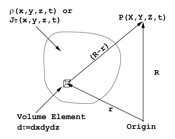
The elementary solution (\ref{7.15}) of the wave equation can be used, together with the principle of superposition, to construct a particular solution of the wave equation given a space and time varying distribution of charge density (see Figure (7.2.1)):

\[\text{V}(\vec{\text{R}}, \text{t})=\frac{1}{4 \pi \epsilon_{0}} \int \int \int_{S p a c e} \text{d} \tau \frac{\rho_{T}\left(\vec{\text{r}}, \text{t}_{\text{R}}\right)}{|\vec{\text{R}}-\vec{\text{r}}|} , \label{7.16}\]

where d\(\tau\) is the element of volume and the retarded time is given by

\[\text{t}_{\text{R}}=\text{t}-\frac{|\vec{\text{R}}-\vec{\text{r}}|}{\text{c}} , \label{7.17}\]

It may be helpful to write out Equation (\ref{7.16}) explicitly in cartesian co-ordinates (see Figure (7.2.1):

\[\text{V}_{\text{P}}(\text{X}, \text{Y}, \text{Z}, \text{t})=\frac{1}{4 \pi \epsilon_{0}} \int \int \int_{S p a \alpha e} \operatorname{dxdydz} \frac{\rho_{T}\left(\text{x}, \text{y}, \text{z}, \text{t}_{\text{R}}\right)}{\sqrt{(\text{X}-\text{x})^{2}+(\text{Y}-\text{y})^{2}+(\text{Z}-\text{z})^{2}}} , \nonumber \]

where

\[\text{t}_{\text{R}}=\text{t}-\frac{\sqrt{(\text{X}-\text{x})^{2}+(\text{Y}-\text{y})^{2}+(\text{Z}-\text{z})^{2}}}{\text{c}}, \nonumber \]

If Equation (\ref{7.16}) is the required solution of the inhomogeneous wave equation (\ref{7.12}) for the potential function \(\text{V}(\vec{\text{R}}, \text{t})\), then by analogy the solution of each of the three Equations (\ref{7.11}) must have the same form. The particular solution for the vector potential that is generated by the current density \(\vec{\text{J}}_{T}(\vec{\text{r}}, t)\) is given by

\[\vec{\text{A}}(\vec{\text{R}}, \text{t})=\frac{\mu_{0}}{4 \pi} \int \int \int_{S p a c e} \text{d} \tau \frac{\vec{\text{J}}_{T}\left(\vec{\text{r}}, \text{t}_{\text{R}}\right)}{|\vec{\text{R}}-\vec{\text{r}}|} . \label{7.18}\]

Here again t_R is the retarded time. These solutions, which satisfy Maxwell’s equations for the case in which the charge and current distributions depend upon time, have exactly the same form as the solution for the electrostatic potential, Equation (2.2.4), and the solution for the magnetostatic vector potential, Equation (4.1.13), except that the retarded time must be used in the source terms. The presence of the retarded time in the integrals makes the calculation of the scalar and vector potentials much more complicated than the equivalent calculations for the static limit. It can be shown, after much work, that the potential functions (\ref{7.16}) and (\ref{7.18}) satisfy the Lorentz condition, Equation (\ref{7.9}).