Physics LibreTexts

8.2: Poynting’s Theorem

  • Page ID
    22840
  • \( \newcommand{\vecs}[1]{\overset { \scriptstyle \rightharpoonup} {\mathbf{#1}} } \) \( \newcommand{\vecd}[1]{\overset{-\!-\!\rightharpoonup}{\vphantom{a}\smash {#1}}} \)\(\newcommand{\id}{\mathrm{id}}\) \( \newcommand{\Span}{\mathrm{span}}\) \( \newcommand{\kernel}{\mathrm{null}\,}\) \( \newcommand{\range}{\mathrm{range}\,}\) \( \newcommand{\RealPart}{\mathrm{Re}}\) \( \newcommand{\ImaginaryPart}{\mathrm{Im}}\) \( \newcommand{\Argument}{\mathrm{Arg}}\) \( \newcommand{\norm}[1]{\| #1 \|}\) \( \newcommand{\inner}[2]{\langle #1, #2 \rangle}\) \( \newcommand{\Span}{\mathrm{span}}\) \(\newcommand{\id}{\mathrm{id}}\) \( \newcommand{\Span}{\mathrm{span}}\) \( \newcommand{\kernel}{\mathrm{null}\,}\) \( \newcommand{\range}{\mathrm{range}\,}\) \( \newcommand{\RealPart}{\mathrm{Re}}\) \( \newcommand{\ImaginaryPart}{\mathrm{Im}}\) \( \newcommand{\Argument}{\mathrm{Arg}}\) \( \newcommand{\norm}[1]{\| #1 \|}\) \( \newcommand{\inner}[2]{\langle #1, #2 \rangle}\) \( \newcommand{\Span}{\mathrm{span}}\)\(\newcommand{\AA}{\unicode[.8,0]{x212B}}\)

    A relation between energy flow and energy stored in the electromagnetic field can be obtained from Maxwell’s equations and the vector identity

    \[\operatorname{div}(\vec{\text{E}} \times \vec{\text{H}})=\vec{\text{H}} \cdot \operatorname{curl}(\vec{\text{E}})-\vec{\text{E}} \cdot \operatorname{curl}(\vec{\text{H}}). \label{8.1}\]

    Multiply the Maxwell equation

    \[\operatorname{curl}(\vec{\text{E}})=-\frac{\partial \vec{\text{B}}}{\partial \text{t}} \nonumber \]

    by \(\vec H\), and multiply

    \[\operatorname{curl}(\vec{\text{H}})=\vec{\text{J}}_{f}+\frac{\partial \vec{\text{D}}}{\partial \text{t}} \nonumber \]

    by \(\vec E\) and subtract to obtain

    \[\vec{\text{H}} \cdot \operatorname{curl}(\vec{\text{E}})-\vec{\text{E}} \cdot \operatorname{curl}(\vec{\text{H}})=-\vec{\text{H}} \cdot \frac{\partial \vec{\text{B}}}{\partial \text{t}}-\vec{\text{J}}_{f} \cdot \vec{\text{E}}-\vec{\text{E}} \cdot \frac{\partial \vec{\text{D}}}{\partial \text{t}}. \label{8.2}\]

    Using the identity (\ref{8.1}) this may be rewritten

    \[-\operatorname{div}(\vec{\text{E}} \times \vec{\text{H}})=\vec{\text{J}}_{f} \cdot \vec{\text{E}}+\vec{\text{E}} \cdot \frac{\partial \vec{\text{D}}}{\partial \text{t}}+\vec{\text{H}} \cdot \frac{\partial \vec{\text{B}}}{\partial \text{t}} . \nonumber \]

    Integrate the latter equation over a volume V bounded by a closed surface S. The volume integral over the divergence can be converted to a surface integral by means of Gauss’ theorem:

    \[-\int \int \int_{V} d \tau d i v(\vec{E} \times \vec{H})=-\iint_{S} d S(\vec{E} \times \vec{H}) \cdot \hat{u}_{n} , \nonumber \]

    where dS is an element of surface area, and \(\widehat{\text{u}}_{n}\) is a unit vector normal to dS. Using Gauss’ Theorem one obtains

    \[-\iint_{\text{S}} \text{dS}(\vec{\text{E}} \times \vec{\text{H}}) \cdot \hat{\text{u}}_{n}=\iiint_{V} \text{d} \tau\left(\vec{\text{J}}_{f} \cdot \vec{\text{E}}+\vec{\text{E}} \cdot \frac{\partial \vec{\text{D}}}{\partial \text{t}}+\vec{\text{H}} \cdot \frac{\partial \vec{\text{B}}}{\partial \text{t}}\right) . \label{8.3}\]

    Equation (\ref{8.3}) is the statement of Poynting’s theorem. Each term in (\ref{8.3}) has the units of a rate of change of energy density. The quantity

    \[\vec{\text{S}}=\vec{\text{E}} \times \vec{\text{H}} \label{8.4}\]

    is called Poynting’s vector; it is a measure of the momentum density carried by the electromagnetic field. Momentum density in the field is given by

    \[\vec{\text{g}}=\frac{\vec{\text{S}}}{\text{c}^{2}} ; \nonumber \]

    see the Feynman Lectures on Physics, Volume(II), Chapter(27); ( R.P.Feynman, R.B.Leighton, and M.Sands, Addison-Wesley, Reading, Mass., 1964 ).

    The surface integral of the Poynting vector, \(\vec S\), over any closed surface gives the rate at which energy is transported by the electromagnetic field into the volume bounded by that surface. The three terms on the right hand side of Equation (\ref{8.3}) describe how the energy carried into the volume is distributed.

    These three terms are:

    \(\text { (1) } \iiint_{V} d \tau\left(\vec{J}_{f} \cdot \vec{E}\right) \nonumber \)

    This term describes the rate at which mechanical energy in the system defined by the volume V increases due to the mechanical forces exerted on charged particles by the electric field: it describes the conversion of electric and magnetic energy into kinetic energy and heat. This can be understood by considering the force on a charged particle

    \[\vec{\text{f}}=\text{q}(\vec{\text{E}}+(\vec{\text{v}} \times \vec{\text{B}})) . \nonumber \]

    The rate at which the electromagnetic field does work on the charged particle is

    \[\frac{\text{dW}}{\text{dt}}=\vec{\text{f}} \cdot \vec{\text{v}} \equiv \text{q} \vec{\text{v}} \cdot \vec{\text{E}} . \label{8.5}\]

    (The magnetic field makes no contribution to the work done on the particle because the magnetic force is perpendicular to the velocity, \(\vec v\)). When summed over all the charges in a volume element, Equation (\ref{8.5}) gives, per unit volume, \(\vec{\text{J}}_{f} \cdot \vec{\text{E}}\).

    \(\text { (2) } \int \int \int_{V} \text{d} \tau\left(\vec{\text{E}} \cdot \frac{\partial \vec{\text{D}}}{\partial \text{t}}\right)\)

    This term gives the rate at which the energy stored in the macroscopic electric field increases with time. Its effect can be represented by the rate of increase of an energy density WE:

    \[\frac{\partial \text{W}_{\text{E}}}{\partial \text{t}}=\vec{\text{E}} \cdot \frac{\partial \vec{\text{D}}}{\partial \text{t}} . \label{8.6}\]

    Notice that this term depends upon the properties of the material because it involves the polarization vector through the displacement vector \(\vec{\text{D}}=\epsilon_{0} \vec{\text{E}}+\vec{\text{P}}\).

    \(\text { (3) } \int \int \int_{V} \text{d} \tau\left(\vec{\text{H}} \cdot \frac{\partial \vec{\text{B}}}{\partial t}\right)\)

    This integral describes the rate of increase of energy stored in the volume V in the form of magnetic energy. It corresponds to a rate of increase of a magnetic energy density WB:

    \[\frac{\partial \text{W}_{\text{B}}}{\partial \text{t}}=\vec{\text{H}} \cdot \frac{\partial \vec{\text{B}}}{\partial \text{t}} .\label{8.7}\]

    Notice that this term involves the properties of the matter in the volume V through the presence of the magnetization density, \(\vec M\), in the definition of \(\vec{\text{H}}=\left(\vec{\text{B}} / \mu_{0}\right)-\vec{\text{M}}\).

    Let us apply Poynting’s theorem, Equation (8.3), to a spherical surface surrounding the dipole radiator of Chapter(7). Suppose that the radius of the sphere, R, is so large that only the radiation fields have an appreciable amplitude on its surface; recall that the radiation fields fall off with distance like 1/R (see Equations (7.33)) , whereas the other field components fall off like 1/R2 or 1/R3 . For the case of dipole radiation in free space the Poynting vector has only an r-component because \(\vec E\), \(\vec H\) are perpendicular to one another and also perpendicular to the direction specified by the unit vector \(\hat{\text{u}}_{r}=\vec{\text{r}} / \text{r}\). In free space \(\vec{\text{B}}=\mu_{0} \vec{\text{H}}\) and

    \[\text{S}_{\text{r}}=\frac{\text{E}_{\theta} \text{B}_{\phi}}{\mu_{0}}=\frac{1}{\text{c} \mu_{0}}\left(\frac{1}{4 \pi \epsilon_{0}}\right)^{2}\left(\frac{\text{d}^{2} \text{p}_{\text{z}}}{\text{dt}^{2}}\right)_{\text{t}_{\text{R}}}^{2}\left(\frac{\sin ^{2} \theta}{\text{c}^{4} \text{R}^{2}}\right) , \label{8.8}\]

    where as usual tR = t − R/c is the retarded time. Now take pz = p0 cos (ωt) so that

    \[\left(\frac{\text{d}^{2} \text{p}_{z}}{\text{dt}^{2}}\right)_{\text{tr}}=-\omega^{2} \text{p}_{0} \cos \left(\omega \text{t}_{\text{R}}\right), \nonumber \]

    and therefore

    \[\text{S}_{\text{r}}=\frac{1}{\text{c} \mu_{0}}\left(\frac{1}{4 \pi \epsilon_{0}}\right)^{2}\left(\frac{\omega}{\text{c}}\right)^{4} \text{p}_{0}^{2} \cos ^{2} \omega(\text{t}-\text{R} / \text{c})\left(\frac{\sin ^{2} \theta}{\text{R}^{2}}\right) . \label{8.9}\]

    The time averaged value of the term cos2 ω(t − R/c) is 1/2 ; also c2 = \(1 /\left(\epsilon_{0} \mu_{0}\right)\). These can be used in (\ref{8.9}) to obtain the average rate at which energy is transported through a surface having a radius R:

    \[<\text{S}_{\text{r}}>=\left(\frac{1}{8 \pi}\right)\left(\frac{\text{c}}{4 \pi \epsilon_{0}}\right)\left(\frac{\omega}{\text{c}}\right)^{4} \frac{\text{p}_{0}^{2} \sin ^{2} \theta}{\text{R}^{2}} .\label{8.10}\]

    Eqn.(\ref{8.10}) gives the angular distribution of the time-averaged power radiated by an oscillating electric dipole. The power radiated along the direction of the dipole is zero, and the maximum power is radiated in the plane perpendicular to the dipole (see Figure (8.1.1)). The total average power radiated by the dipole can be obtained by integrating (\ref{8.10}) over the surface of the sphere of radius R:
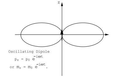
    Figure 8.1.PNG

    Figure \(\PageIndex{1}\): The pattern of radiated power for an oscillating electric dipole. There is no power radiated along the direction of the dipole, \(\vec p\) or \(\vec m\).

    \[\int \int_{Sphere } \text{dS}<\text{S}_{\text{r}}>=\int_{0}^{\pi}<\text{S}_{\text{r}}>2 \pi \text{R}^{2} \sin \theta \text{d} \theta=\frac{\text{c}}{16 \pi \epsilon_{0}}\left(\frac{\omega}{\text{c}}\right)^{4} \text{p}_{0}^{2} \int_{0}^{\pi} \sin ^{3} \theta \text{d} \theta. \nonumber \]

    But \(\int_{0}^{\pi} \sin ^{3} \theta \text{d} \theta=4 / 3\) so that the total average power radiated by the oscillating electric dipole is given by

    \[P_{E}=\frac{1}{3} \frac{c}{4 \pi \epsilon_{0}}\left(\frac{\omega}{c}\right)^{4} p_{0}^{2} \quad W a t t s. \label{8.11}\]

    The rate of energy radiated by the dipole increases very rapidly with the frequency for a fixed dipole moment, p0.

    A similar calculation gives the average rate, PM, at which energy is radiated by an oscillating magnetic dipole. The far fields generated by an oscillating magnetic dipole are given by

    \[\text{B}_{\theta}=\frac{\mu_{0}}{4 \pi}\left(\frac{\text{d}^{2} \text{m}_{z}}{\text{dt}^{2}}\right)_{\text{t}_{\text{R}}} \frac{\sin \theta}{\text{c}^{2} \text{R}}, \nonumber \]

    Figure 8.2.PNG
    Figure \(\PageIndex{2}\): The schematic diagram of a center-fed, linear, half-wave antenna oriented along the z-axis. The current is zero at the ends of the antenna; these are located at z=-L and at z=+L.

    \[\text{E}_{\phi}=-\text{c B}_{\theta} , \nonumber \]

    where as usual tR = t − R/c is the retarded time. For a magnetic dipole whose amplitude is m0 one finds

    \[\text{P}_{\text{M}}=\frac{\text{c}}{3} \frac{\mu_{0}}{4 \pi}\left(\frac{\omega}{\text{c}}\right)^{4} \text{m}_{0}^{2} \quad \text { Watts }. \label{8.12}\]


    This page titled 8.2: Poynting’s Theorem is shared under a CC BY 4.0 license and was authored, remixed, and/or curated by John F. Cochran and Bretislav Heinrich.