
13.9D: Bridge Solution by Delta-Star Transform


- Last updated
- Mar 5, 2022
- Save as PDF

( \newcommand{\kernel}{\mathrm{null}\,}\)
In the above examples, we have calculated the condition that there is no current in the detector -. i.e. that the bridge is balanced. Such calculations are relatively easy. But what if the bridge is not balanced? Can we calculate the impedance of the circuit? Can we calculate the currents in each branch, or the potentials at any points? This is evidently a little harder. We should be able to do it. Kirchhoff’s rules and the delta-star transform still apply for alternating currents, the complication being that all impedances, currents and potentials are complex numbers.
Let us start by trying the following problem:
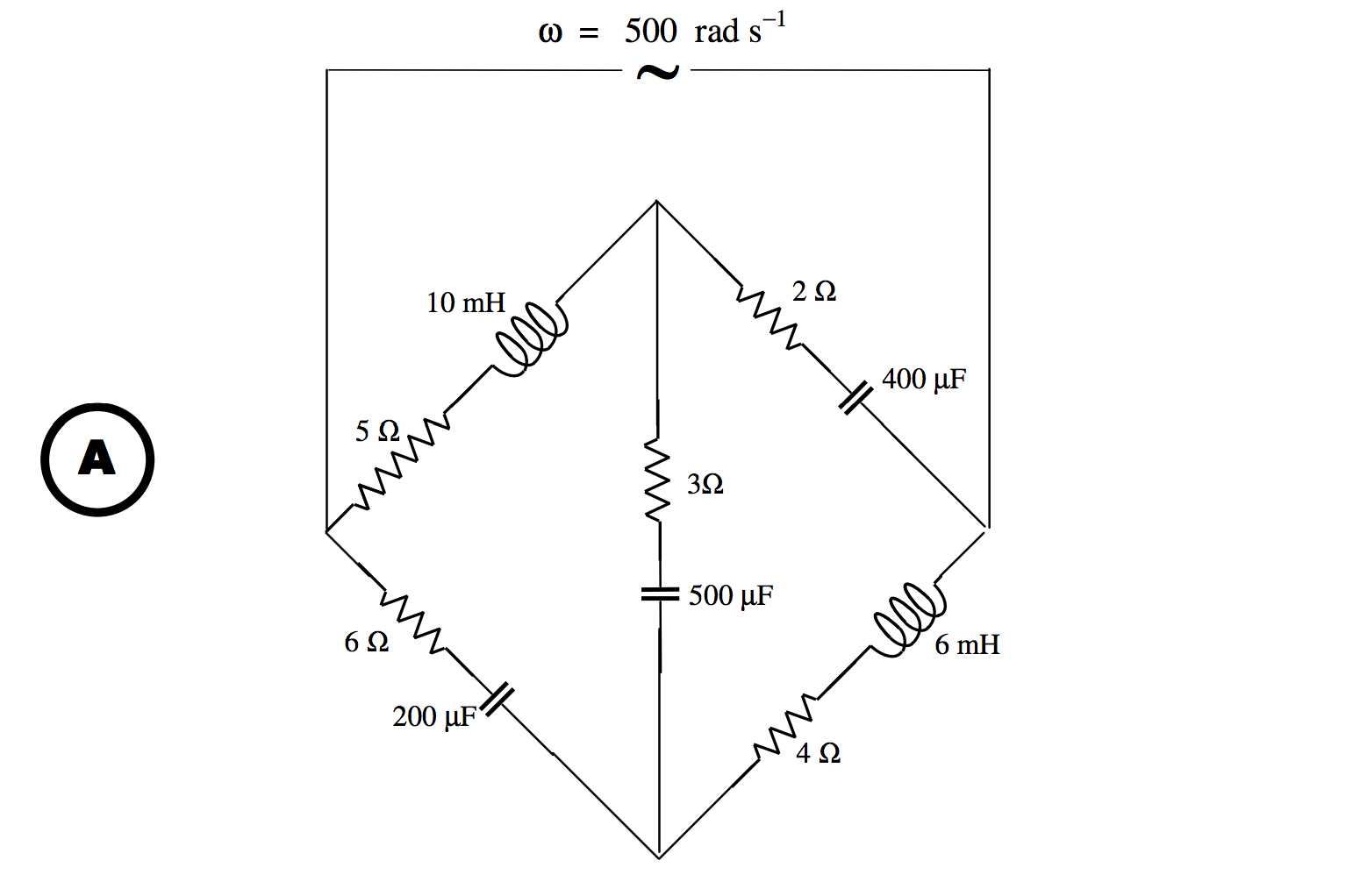
That is to say:
*The impedances are indicated in ohms.
Our question is: What is the impedance of the circuit at a frequency of ω=500 rad s−1?
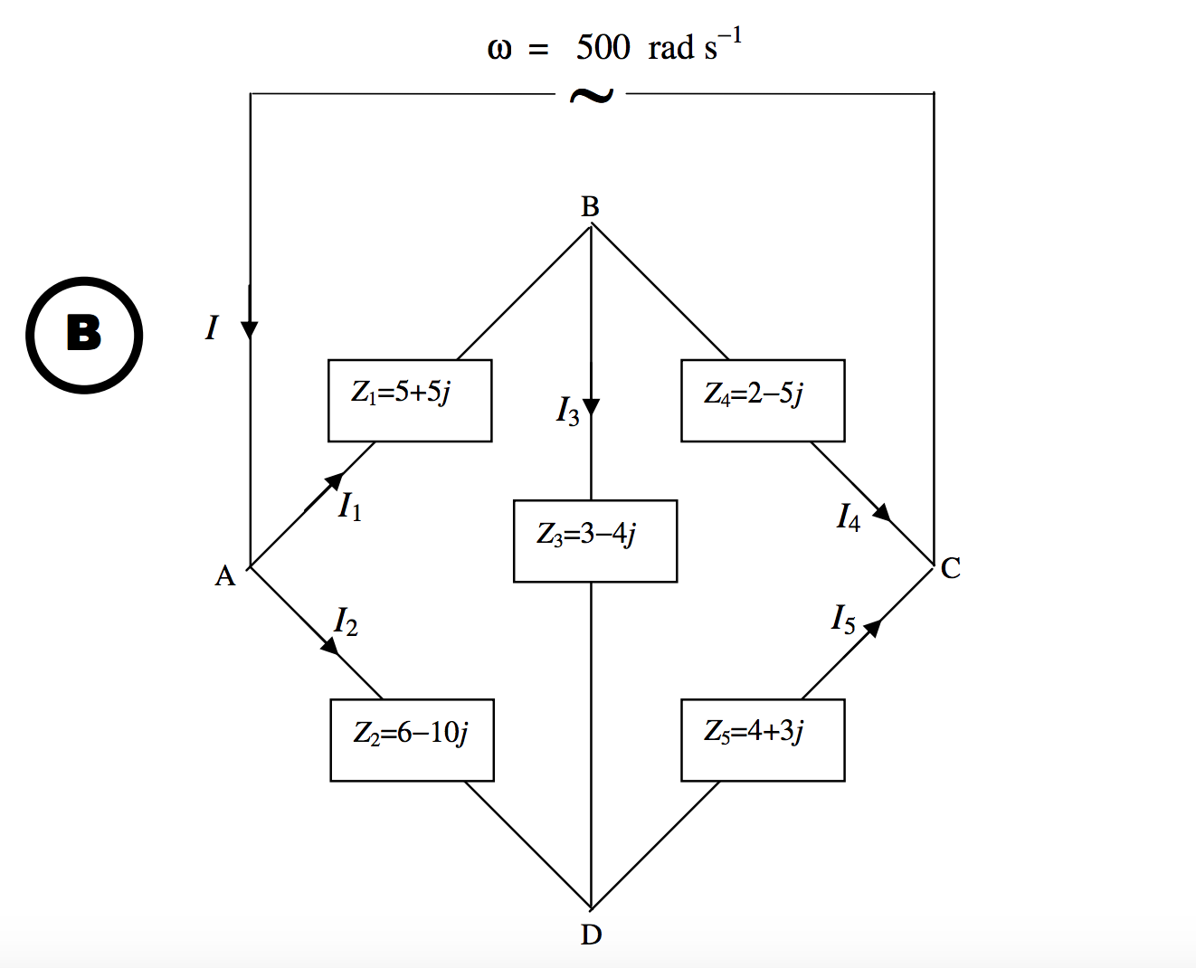
We refer now to Chapter 4, Section 12. We are going to replace the left hand “delta” with its equivalent “star”. Recall equations 4.12.2 - 4.12.13. With alternating currents, We can use the same equations with alternating currents, provided that we replace the R1R2R3G1G2G3 in the delta and the r1r2r3g1g2g3 in the star with Z1Z2Z3Y1Y2Y3 in the delta and z1z2z3y1y2y3 in the star. That is, we replace the resistances with impedances, and conductances with admittances. This is going to need a little bit of calculation, and familiarity with complex numbers. I used a computer - hand calculation was too tedious and prone to mistakes. This is what I got, using z1=Z2Z3Z1+Z2+Z3 and cyclic variations:
*The impedances are indicated in ohms.
z1=0.642599−3.444043jz2=1.931408+0.884477jz3=4.693141+1.588448j
- The impedance of PBC is 3.931408−4.115523jΩ.
- The impedance of PDC is 4.642599−0.444043jΩ.
- The admittance of PBC is 0.121364+0.127048jS.
- The admittance of PDC is 0.213444+0.020415jS.
- The admittance of PC is 0.334808+0.147463jS.
- The impedance of PC is 2.501523−1.101770jΩ.
- The impedance of AC is 7.194664+0.486678jΩ_.
- The admittance of AC is 0.138359−0.009359jS.
Suppose the applied voltage is V=VA−VC=ˆVcosωt, with ω=500 rad s−1 and ˆV=24V.
Can we find the currents in each of Z1,Z2,Z3,Z4,Z5, and the potential differences between the several points? This should be fun. I’m sitting in front of my computer. Among other things, I have trained it instantly to multiply two complex numbers and also to calculate the reciprocal of a complex number. If I ask it for (2.3+4.1j)(1.9−3.4j) it will instantly tell me 18.31−0.03j. If I ask it for 1/(0.5+1.2j) it will instantly tell me 0.2959−0.7101j. I can instantaneously convert between impedance and admittance.
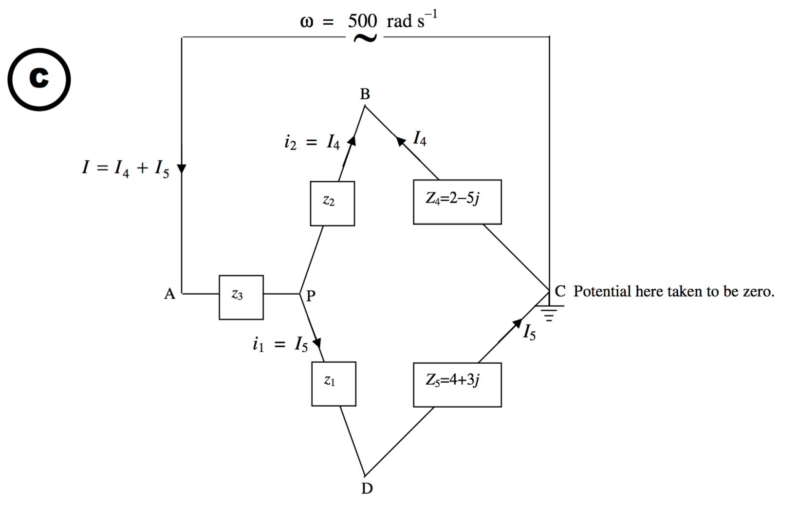
The current through any element depends on the potential difference across it. We can take any point to have zero potential, and determine the potentials at other points relative to that point. I choose to take the potential at C to be zero, and I have indicated this by means of a ground (earth) symbol at C. We are going to try to find the potentials at various other points relative to that at C.
In drawings B and C I have indicated the currents with arrows. Since the currents are alternating, they should, perhaps, be drawn as double-headed arrows. However, I have drawn them in the direction that I think they should be at some instant when the potential at A is greater than the potential at C. If any of my guesses are wrong, I’ll get a negative answer in the usual way.
The total current I is V times the admittance of the circuit.
That is: I=24×(0.138359−0.009359j)=(3.320611−0.224620j)A.
The peak current will be 3.328200 A (because the modulus of the admittance is 0.138675 S), and the current lags behind the voltage by 3º.9.
I hope the following two equations are obvious from drawing C.
I=I4+I5I4(z2+Z4)=I5(z1+Z5)
From this,
I4=(z1+Z5z1+z2+Z4+Z5)I=(4.642599−0.444043j8.574007−4.559567j)×(3.320611−0.224620j)=1.514284+0.511681j_A
I4 leads on V by 18º.7 ˆI4=1.598397A.
I5=(z2+Z4z1+z2+Z4+Z5)I=1.806328−0.736302j A_
I5 lags behind V by 22º.2 ˆI5=1.950631A.
Check: I4+I5=I✓
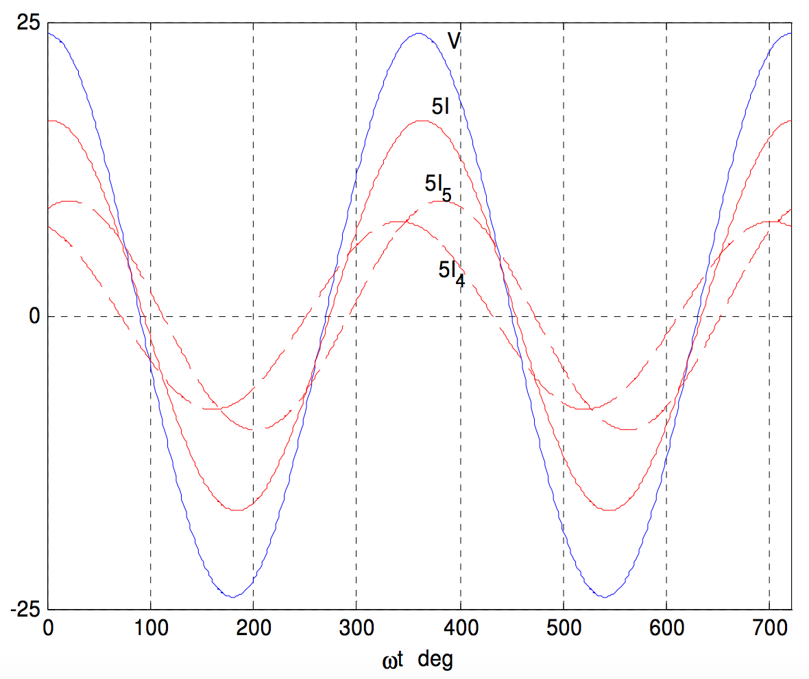
I show below graphs of the potential difference between A and C (V=VA−VC) and the currents I, I4 and I5. The origin for the horizontal scale is such that the potential at A is zero at t=0. The vertical scale is in volts for VC, and is five times the current in amps for the three currents.
We don’t really need to know i1,i2,i3, but we do want to know I1,I2,I3. Let’s first see if we can find some potentials relative to the point C.
From drawing C we see that
VB−VC=VD=I4Z4, which results in VB=(5.586975−6.548057j)V_
VB lags behind V by 0.864432 rad =49º.5 ˆVB=8.607603 V.
From drawing C we see that
VD−VC=VD=I5Z5, which results in VD=(9.434216+2.473775j) V_
VD leads on V by 0.256440 rad = 14º.7 ˆVB=9.753153 V.
We can now calculate I3 (see drawing B) from I3=VB−VDZ3=(VB−VD)Y3.
I find I3=0.981824−1.698178j A_
I3 lags behind V by 1.046588 rad = 60º.0. ˆI3=1.961578 A.
I1 can now be found from I1=VA−VBZ1=(VA−VB)Y1. The real part ofVA is 24 V, and (since we have grounded C), its imaginary part is zero. If in doubt about this verify that
IZ=(3.320611−0.224620j)(7.194664+0.486678j)=(24+0j)V.✓
I find
I1=2.496108−1.186497j A_
I1 lags behind V by 0.443725 rad =25º.4. ˆI1=2.763753 A.
In a similar manner, I find
I2=0.824503+0.961876j A_
I2 leads on V by 0.862147 rad = 49º.4. ˆI2=1.266891 A.
Summary:
- I=3.320611−0.224620j A_
- I1=2.496108−1.186497j A_
- I2=0.824503−0.961876j A_
- I3=0.981824−1.698178j A_
- I4=1.514284−0.511681j A_
- I5=1.806328−0.736302j A_
These may be checked by verification of Kirchhoff’s first rule at each of the points A, B, C, D.