2.1: Maxwell’s differential equations in the time domain

Whereas the Lorentz force law characterizes the observable effects of electric and magnetic fields on charges, Maxwell’s equations characterize the origins of those fields and their relationships to each other. The simplest representation of Maxwell’s equations is in differential form, which leads directly to waves; the alternate integral form is presented in Section 2.4.3.

The differential form uses the overlinetor del operator ∇:

\[\nabla \equiv \hat{x} \frac{\partial}{\partial \mathrm{x}}+\hat{y} \frac{\partial}{\partial \mathrm{y}}+\hat{z} \frac{\partial}{\partial \mathrm{z}}\]

where \(\hat{x}, \hat{y}\), and \(\hat{z}\) are defined as unit overlinetors in cartesian coordinates. Relations involving ∇ are summarized in Appendix D. Here we use the conventional overlinetor dot product¹ and cross product² of ∇ with the electric and magnetic field overlinetors where, for example:

\[\overline{\mathrm{E}}=\hat{x} \mathrm{E}_{\mathrm{x}}+\hat{y} \mathrm{E}_{\mathrm{y}}+\hat{z} \mathrm{E}_{\mathrm{z}}\]

\[\nabla \cdot \overline{\mathrm{E}} \equiv \frac{\partial \mathrm{E}_{\mathrm{x}}}{\partial \mathrm{x}}+\frac{\partial \mathrm{E}_{\mathrm{y}}}{\partial \mathrm{y}}+\frac{\partial \mathrm{E}_{\mathrm{z}}}{\partial \mathrm{z}}\]

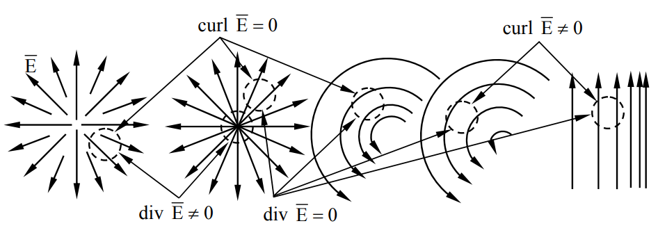
We call \(\nabla \cdot \overline{\mathrm{E}}\) the divergence of E because it is a measure of the degree to which the overlinetor field \(\overline E\) diverges or flows outward from any position. The cross product is defined as:

\[\begin{aligned}
\nabla \times \overline{\mathrm{E}} & \equiv \hat{x}\left(\frac{\partial \mathrm{E}_{\mathrm{z}}}{\partial \mathrm{y}}-\frac{\partial \mathrm{E}_{\mathrm{y}}}{\partial \mathrm{z}}\right)+\hat{y}\left(\frac{\partial \mathrm{E}_{\mathrm{x}}}{\partial \mathrm{z}}-\frac{\partial \mathrm{E}_{\mathrm{z}}}{\partial \mathrm{x}}\right)+\hat{z}\left(\frac{\partial \mathrm{E}_{\mathrm{y}}}{\partial \mathrm{x}}-\frac{\partial \mathrm{E}_{\mathrm{x}}}{\partial \mathrm{y}}\right) \\
&=\operatorname{det}\left|\begin{array}{ccc}
\hat{x} & \hat{y} & \hat{z} \\
\partial / \partial \mathrm{x} & \partial / \partial \mathrm{y} & \partial / \partial \mathrm{z} \\
\mathrm{E}_{\mathrm{x}} & \mathrm{E}_{\mathrm{y}} & \mathrm{E}_{\mathrm{z}}
\end{array}\right|
\end{aligned}\]

which is often called the curl of E . Figure 2.1.1 illustrates when the divergence and curl are zero or non-zero for five representative field distributions.

¹ The dot product of \(\overline A\) and \(\overline B\) can be defined as \(\bar{A} \cdot \bar{B}=A_{x} B_{x}+A_{y} B_{y}+A_{z} B_{z}=|A||B| \cos \theta\), where θ is the angle between the two overlinetors.

² The cross product of \(\overline A\) and \(\overline B\) can be defined as \(\bar{A} \times \bar{B}=\hat{x}\left(A_{y} B_{z}-A_{z} B_{y}\right)+\hat{y}\left(A_{z} B_{x}-A_{x} B_{z}\right)+\hat{z}\left(\mathrm{A}_{\mathrm{x}} \mathrm{B}_{\mathrm{y}}-\mathrm{A}_{\mathrm{y}} \mathrm{B}_{\mathrm{x}}\right)\); its magnitude is \(|\overline{\mathrm{A}}| \cdot|\overline{\mathrm{B}}| \sin \theta\). Alternatively, \(\overline{\mathrm{A}} \times \overline{\mathrm{B}}=\operatorname{det}\left|\left[\mathrm{A}_{\mathrm{x}}, \mathrm{A}_{\mathrm{y}}, \mathrm{A}_{\mathrm{z}}\right],\left[\mathrm{B}_{\mathrm{x}}, \mathrm{B}_{\mathrm{y}}, \mathrm{B}_{\mathrm{z}}\right],[\hat{x}, \hat{y}, \hat{z}]\right|\).

Figure 2.1.1: Fields with zero or non-zero divergence or curl.

The differential form of Maxwell’s equations in the time domain are:

\[\nabla \times \overline{\mathrm{E}}=-\frac{\partial \overline{\mathrm{B}}}{\partial \mathrm{t}} \quad \quad \quad \quad \text { Faraday's Law }\]

\[\nabla \times \overline{\mathrm{H}}=\overline{\mathrm{J}}+\frac{\partial \overline{\mathrm{D}}}{\partial \mathrm{t}} \quad \quad \quad \quad \text { Ampere's Law }\]

\[\nabla \bullet \overline{\mathrm{D}}=\rho \quad \quad \quad \quad \text {Gauss’s Law}\]

\[\nabla \cdot \overline{\mathrm{B}}=0 quad \quad \quad \quad \text {Gauss’s Law}\]

The field variables are defined as:

\[\overline{\mathrm{E}} \quad \text{electric field}\quad \quad \quad \quad \quad {[volts/meter; Vm^{-1}] }\]

\[ \overline{\mathrm{H}} \quad \text{magnetic field}\quad \quad \quad \quad \quad {[amperes/meter; Am^{-1}] }\]

\[\overline{\mathrm{B}} \quad \text{magnetic flux density }\quad \quad \quad \quad \quad {[Tesla; T] } \]

\[ \overline{\mathrm{D}} \quad \text{electric displacement }\quad \quad \quad \quad \quad {[coulombs/m^2; Cm^{-2}] }\]

\[\overline{\mathrm{J}} \quad \text{electric current density }\quad \quad \quad \quad \quad {[amperes/m^2; Am^{-2}] } \]

\[\overline{\mathrm{\rho}} \quad \text{electric charge density }\quad \quad \quad \quad \quad {[coulombs/m^3; Cm^{-3}]} \]

These four Maxwell equations invoke one scalar and five overlinetor quantities comprising 16 variables. Some variables only characterize how matter alters field behavior, as discussed later in Section 2.5. In vacuum we can eliminate three overlinetors (9 variables) by noting:

\[\overline{\mathrm{D}}=\varepsilon_{\mathrm{o}} \overline{\mathrm{E}} \quad \quad \quad \quad \quad {(constitutive \ relation \ for \ \overline{D} ) } \]

\[ \overline{\mathrm{B}}=\mu_{\mathrm{o}} \overline{\mathrm{H}} \quad \quad \quad \quad \quad {(constitutive \ relation \ for \ \overline{B} ) }\]

\[ \overline{\mathrm{J}}=\rho \overline{\mathrm{v}}=\sigma \overline{\mathrm{E}} \quad \quad \quad \quad \quad {(constitutive \ relation \ for \ \overline{J} )}\]

where ε_o = 8.8542×10^-12 [farads m^-1] is the permittivity of vacuum, μ_o = 4\(\pi\)×10^-7 [henries m^-1] is the permeability of vacuum³ , v is the velocity of the local net charge density ρ, and σ is the conductivity of a medium [Siemens m^-1]. If we regard the electrical sources ρ and J as given, then the equations can be solved for all remaining unknowns. Specifically, we can then find E and H , and thus compute the forces on all charges present. Except for special cases we shall avoid solving problems where the electromagnetic fields and the motions of ρ are interdependent.

The constitutive relations for vacuum, \(\mathrm{D}=\varepsilon_{0} \overline{\mathrm{E}} \) and \( \overline{\mathrm{B}}=\mu_{0} \overline{\mathrm{H}}\), can be generalized to \( \overline{\mathrm{D}}=\varepsilon \overline{\mathrm{E}}\), \( \overline{\mathrm{B}}=\mu \overline{\mathrm{H}}\), and \(\overline{\mathrm{J}}=\sigma \overline{\mathrm{E}} \) for simple media. Media are discussed further in Section 2.5.

Maxwell’s equations require conservation of charge. By taking the divergence of Ampere’s law (2.1.6) and noting the overlinetor identity \(\nabla \bullet(\nabla \times \overline{\mathrm{A}})=0 \), we find:

\[ \nabla \bullet(\nabla \times \bar{H})=0=\nabla \bullet \frac{\partial \bar{D}}{\partial t}+\nabla \bullet \bar{J}\]

Then, by reversing the sequence of the derivatives in (2.1.18) and substituting Gauss’s law \( \nabla \bullet \overline{\mathrm{D}}=\rho\) (2.1.7), we obtain the differential expression for conservation of charge:

\[ \nabla \bullet \overline{\mathrm{J}}=-\frac{\partial \rho}{\partial \mathrm{t}} \quad \quad \quad \quad \quad \text{(conservation of charge)}\]

The integral expression can be derived from the differential expression by using Gauss’s divergence theorem, which relates the integral of \( \nabla \bullet \bar{G}\) over any volume V to the integral of \(\overline{\mathrm{G}} \bullet \hat{n} \) over the surface area A of that volume, where the surface normal unit overlinetor \(\hat{n} \) points outward:

\[\int \int \int_{V} \nabla \bullet \bar{G} d v=\oiint_{A} \bar{G} \bullet \hat{n} d a \quad \quad \quad \quad \quad \text{(Gauss’s divergence theorem)} \]

Thus the integral expression for conservation of charge is:

\[\frac{\mathrm{d}}{\mathrm{dt}} \int \int \int_{\mathrm{V}} \rho \mathrm{d} \mathrm{v}=-\oiint_{\mathrm{A}} \overline{\mathrm{J}} \bullet \hat{n} \mathrm{d} \mathrm{a} \quad \quad \quad \quad \quad \text{(conservation of charge)} \]

which says that if no net current \(\overline J\) flows through the walls A of a volume V, then the total charge inside must remain constant.

³ The constant 4\(\pi\) × 10^-7 is exact and enters into the definition of an ampere.

Example \(\PageIndex{A}\)

If the electric field in vacuum is \(\overline{\mathrm{E}}=\hat{x} \mathrm{E}_{\mathrm{o}} \cos (\omega \mathrm{t}-\mathrm{ky})\), what is \(\overline H\)?

Solution

From Faraday’s law (2.1.5): \(\mu_{0}(\partial \overline{\mathrm{H}} / \partial \mathrm{t})=-(\nabla \times \overline{\mathrm{E}})=\hat{z} \partial \mathrm{E}_{\mathrm{x}} / \partial \mathrm{y}=\hat{z} \mathrm{kE}_{\mathrm{o}} \sin (\omega \mathrm{t}-\mathrm{ky})\), using (2.1.4) for the curl operator. Integration of this equation with respect to time yields: \(\overline{\mathrm{H}}=-\hat{z}\left(\mathrm{kE}_{\mathrm{o}} / \mu_{\mathrm{o}} \omega\right) \cos (\omega \mathrm{t}-\mathrm{ky})\).

Example \(\PageIndex{B}\)

Does the electric field in vacuum \(\overline{\mathrm{E}}=\hat{x} \mathrm{E}_{\mathrm{o}} \cos (\omega \mathrm{t}-\mathrm{kx})\) satisf y Maxwell’s equations? Under what circumstances would this \(\overline E\) satisfy the equations?

Solution

This electric field does not satisfy Gauss’s law for vacuum, which requires \(\nabla \bullet \overline{\mathrm{D}}=\rho=0\). It satisfies Gauss’s law only for non-zero charge density: \(\rho=\nabla \bullet \overline{\mathrm{D}}=\varepsilon_{\mathrm{o}} \partial \mathrm{E}_{\mathrm{x}} / \partial \mathrm{x}=\partial\left[\varepsilon_{\mathrm{o}} \mathrm{E}_{\mathrm{o}} \cos (\omega \mathrm{t}-\mathrm{kx})\right] / \partial \mathrm{x}=\mathrm{k} \varepsilon_{\mathrm{o}} \mathrm{E}_{\mathrm{o}} \sin (\omega \mathrm{t}-\mathrm{kx}) \neq 0\). To satisfy the remaining Maxwell equations and conservation of charge (2.1.19) there must also be a current \(\overline{\mathrm{J}} \neq 0\) corresponding to \(\rho: \overline{\mathrm{J}}=\sigma \overline{\mathrm{E}}=\hat{x} \sigma \mathrm{E}_{\mathrm{o}} \cos (\omega \mathrm{t}-\mathrm{kx})\), where (2.1.17) simplified the computation.