Physics LibreTexts

2.7: Power and Energy in the Time and Frequency Domains and the Poynting Theorem

  • Page ID
    24992
  • \( \newcommand{\vecs}[1]{\overset { \scriptstyle \rightharpoonup} {\mathbf{#1}} } \) \( \newcommand{\vecd}[1]{\overset{-\!-\!\rightharpoonup}{\vphantom{a}\smash {#1}}} \)\(\newcommand{\id}{\mathrm{id}}\) \( \newcommand{\Span}{\mathrm{span}}\) \( \newcommand{\kernel}{\mathrm{null}\,}\) \( \newcommand{\range}{\mathrm{range}\,}\) \( \newcommand{\RealPart}{\mathrm{Re}}\) \( \newcommand{\ImaginaryPart}{\mathrm{Im}}\) \( \newcommand{\Argument}{\mathrm{Arg}}\) \( \newcommand{\norm}[1]{\| #1 \|}\) \( \newcommand{\inner}[2]{\langle #1, #2 \rangle}\) \( \newcommand{\Span}{\mathrm{span}}\) \(\newcommand{\id}{\mathrm{id}}\) \( \newcommand{\Span}{\mathrm{span}}\) \( \newcommand{\kernel}{\mathrm{null}\,}\) \( \newcommand{\range}{\mathrm{range}\,}\) \( \newcommand{\RealPart}{\mathrm{Re}}\) \( \newcommand{\ImaginaryPart}{\mathrm{Im}}\) \( \newcommand{\Argument}{\mathrm{Arg}}\) \( \newcommand{\norm}[1]{\| #1 \|}\) \( \newcommand{\inner}[2]{\langle #1, #2 \rangle}\) \( \newcommand{\Span}{\mathrm{span}}\)\(\newcommand{\AA}{\unicode[.8,0]{x212B}}\)

    Poynting theorem and definition of power and energy in the time domain

    To derive the Poynting theorem we can manipulate Maxwell’s equations to produce products of variables that have the dimensions and character of power or energy. For example, the power dissipated in a resistor is the product of its voltage and current, so the product \(\overline{\mathrm{E}} \bullet \overline{\mathrm{J}}\left[\mathrm{W} \mathrm{m}^{-3}\right]\) would be of interest. The dimensions of \(\overline E\) and \(\overline J\) are volts per meter and amperes per square meter, respectively. Faraday’s and Ampere’s laws are:

    \[\nabla \times \overline{\mathrm{E}}=-\frac{\partial \overline{\mathrm{B}}}{\partial \mathrm{t}} \quad \quad \quad \quad \quad \text { (Faraday's law) } \]

    \[ \nabla \times \overline{H}=\overline{J}+\frac{\partial \overline{D}}{\partial t} \quad \quad \quad \quad \quad \text { (Ampere's law) }\]

    We can produce the product \(\overline{E} \bullet \overline{J} \) and preserve symmetry in the resulting equation by taking the dot product of \(\overline E\) with Ampere’s law and subtracting from it the dot product of \(\overline H\) with Faraday’s law, yielding:

    \[\begin{align}
    \overline{\mathrm{E}} \bullet(\nabla \times \overline{\mathrm{H}})-\overline{\mathrm{H}} \bullet(\nabla \times \overline{\mathrm{E}}) &=\overline{\mathrm{E}} \bullet \overline{\mathrm{J}}+\overline{\mathrm{E}} \bullet \frac{\partial \overline{\mathrm{D}}}{\partial \mathrm{t}}+\overline{\mathrm{H}} \bullet \frac{\partial \overline{\mathrm{B}}}{\partial \mathrm{t}} \\ &=-\nabla \bullet(\overline{\mathrm{E}} \times \overline{\mathrm{H}}) \end{align} \]

    where (2.7.4) is a overlinetor identity. Equations (2.7.3) and (2.7.4) can be combined to form the Poynting theorem:

    \[ \nabla \bullet(\overline{E} \times \overline{H})+\overline{E} \bullet \overline{J}+\overline{E} \bullet \frac{\partial \overline{D}}{\partial t}+\overline{H} \bullet \frac{\partial \overline{B}}{\partial t}=0 \ \left[W m^{-3}\right]\]

    The dimension of \(\overline{E} \bullet \overline{J} \) and every other term in this equation is W m-3. If \( \overline{\mathrm{D}}=\varepsilon \overline{\mathrm{E}}\) and \(\overline{\mathrm{B}}=\mu \overline{\mathrm{H}} \), then \( \overline{\mathrm{E}} \bullet \partial \overline{\mathrm{D}} / \partial \mathrm{t}=\partial\left[\varepsilon|\overline{\mathrm{E}}|^{2} / 2\right] / \partial \mathrm{t}\) and \( \overline{\mathrm{H}} \bullet \partial \overline{\mathrm{B}} / \partial \mathrm{t}=\partial\left[\mu|\overline{\mathrm{H}}|^{2} / 2\right] / \partial \mathrm{t}\). The factor of one-half arises because we are now differentiating with respect to a squared quantity rather than a single quantity, as in (2.7.5). It follows that \( \varepsilon|\overrightarrow{\mathrm{E}}|^{2} / 2\) and \(\mu|\overrightarrow{\mathrm{H}}|^{2} / 2 \) have the dimension of J m-3 and represent electric and magnetic energy density, respectively, denoted by We and Wm. The product \(\overline{E} \bullet \overline{J} \) can represent either power dissipation or a power source, both denoted by Pd. If \(\overline{\mathrm{J}}=\sigma \overline{\mathrm{E}} \), then \( \mathrm{P}_{\mathrm{d}}=\sigma|\overline{\mathrm{E}}|^{2} \ \left[\mathrm{W} \mathrm{m}^{-3}\right]\), where σ is the conductivity of the medium, as discussed later in Section 3.1.2. To summarize:

    \[ P_{d}=\overline{J} \bullet \overline{E} \ \left[W m^{-3}\right] \quad\quad\quad\quad\quad(\text {power dissipation density})\]

    \[\mathrm{W}_{\mathrm{e}}=\frac{1}{2} \varepsilon|\overline{\mathrm{E}}|^{2}\ \left[\mathrm{J} \mathrm{m}^{-3}\right] \quad\quad\quad\quad\quad(\text {electric energy density}) \]

    \[\mathrm{W}_{\mathrm{m}}=\frac{1}{2} \mu|\overline{\mathrm{H}}|^{2} \ \left[\mathrm{J} \mathrm{m}^{-3}\right] \quad\quad\quad\quad\quad(\text { magnetic energy density }) \]

    Thus we can write Poynting’s theorem in a simpler form:

    \[\nabla \bullet(\overline{\mathrm{E}} \times \overline{\mathrm{H}})+\overline{\mathrm{E}} \bullet \overline{\mathrm{J}}+\frac{\partial}{\partial \mathrm{t}}\left(\mathrm{W}_{\mathrm{e}}+\mathrm{W}_{\mathrm{m}}\right)=0 \ \left[\mathrm{Wm}^{-3}\right] \quad \quad \quad \quad \quad \text { (Poynting theorem) } \]

    suggesting that the sum of the divergence of electromagnetic power associated with \( \overline{\mathrm{E}} \times \overline{\mathrm{H}}\), the density of power dissipated, and the rate of increase of energy storage density must equal zero.

    The physical interpretation of \( \nabla \bullet(\overline{E} \times \overline{H})\) is best seen by applying Gauss’s divergence theorem to yield the integral form of the Poynting theorem:

    \[\oiint_{\mathrm{A}}(\overline{\mathrm{E}} \times \overline{\mathrm{H}}) \bullet \hat{n} \mathrm{d} \mathrm{a}+\int \int _{\mathrm{V}} \overline{\mathrm{E}} \bullet \overline{\mathrm{J}} \mathrm{d} \mathrm{v}+(\partial / \partial \mathrm{t}) \int \int \int_{\mathrm{V}} \frac{1}{2}(\overline{\mathrm{E}} \bullet \overline{\mathrm{D}}+\overline{\mathrm{H}} \bullet \overline{\mathrm{B}}) \mathrm{d} \mathrm{v}=0 \ [\mathrm{W}] \]

    which can also be represented as:

    \[ \oiint_{\mathrm{A}}(\overline{\mathrm{E}} \times \overline{\mathrm{H}}) \bullet \hat{n} \mathrm{d} \mathrm{a}+\mathrm{p}_{\mathrm{d}}+\frac{\partial}{\partial \mathrm{t}}\left(\mathrm{w}_{\mathrm{e}}+\mathrm{w}_{\mathrm{m}}\right)=0 \ [\mathrm{W}] \quad \quad \quad \quad \quad \text { (Poynting theorem) }\]

    Based on (2.7.8) and conservation of power (1.1.6) it is natural to associate \( \overline{\mathrm{E}} \times \overline{\mathrm{H}} \ \left[\mathrm{W} \mathrm{m}^{-2}\right]\) with the instantaneous power density of an electromagnetic wave characterized by \(\overline{\mathrm{E}} \ \left[\mathrm{V} \mathrm{m}^{-1}\right] \) and \(\overline{\mathrm{H}} \ \left[\mathrm{A} \mathrm{m}^{-1}\right] \). This product is defined as the Poynting overlinetor:

    \[ \overline{\mathrm{S}} \equiv \overline{\mathrm{E}} \times \overline{\mathrm{H}} \ \left[\mathrm{Wm}^{-2}\right] \quad\quad\quad\quad\quad \text { (Poynting overlinetor) }\]

    The instantaneous electromagnetic wave intensity of a uniform plane wave. Thus Poynting’s theorem says that the integral of the inward component of the Poynting overlinetor over the surface of any volume V equals the sum of the power dissipated and the rate of energy storage increase inside that volume.

    Example \(\PageIndex{A}\)

    Find \(\overline{\mathrm{S}}(\mathrm{t})\) and \( \langle\overline{\mathrm{S}}(\mathrm{t})\rangle\) for a uniform plane wave having \(\overline{\mathrm{E}}=\hat{x} \mathrm{E}_{\mathrm{o}} \cos (\omega \mathrm{t}-\mathrm{kz}) \). Find the electric and magnetic energy densities We(t,z) and Wm(t,z) for the same wave; how are they related?

    Solution

    \(\overline{\mathrm{H}}=\hat{z} \times \overline{\mathrm{E}} / \eta_{\mathrm{o}}=\hat{y} \mathrm{E}_{\mathrm{o}} \cos (\omega \mathrm{t}-\mathrm{kz}) / \eta_{\mathrm{o}} \) where \(\eta_{\mathrm{o}}=\left(\mu_{\mathrm{o}} / \varepsilon_{\mathrm{o}}\right)^{0.5} \). \( \overline{\mathrm{S}}=\overline{\mathrm{E}} \times \overline{\mathrm{H}}=\hat{z} \mathrm{E}_{\mathrm{o}}^{2} \cos ^{2}(\omega \mathrm{t}-\mathrm{kz}) / \eta_{\mathrm{o}}\) and \( \langle\overline{\mathrm{S}}(\mathrm{t})\rangle=\hat{z} \mathrm{E}_{\mathrm{o}}^{2} / 2 \eta_{\mathrm{o}} \ \left[\mathrm{Wm}^{-2}\right]\). \( \mathrm{W}_{\mathrm{e}}(\mathrm{t}, \mathrm{z})=\varepsilon_{\mathrm{o}} \mathrm{E}_{\mathrm{o}}^{2} \cos ^{2}(\omega \mathrm{t}-\mathrm{kz}) / 2 \ \left[\mathrm{Jm}^{-3}\right]\) and \( \mathrm{W}_{\mathrm{m}}(\mathrm{t}, \mathrm{z})=\mu_{\mathrm{o}} \mathrm{E}_{\mathrm{o}}^{2} \cos ^{2}(\omega \mathrm{t}-\mathrm{kz}) / 2 \eta_{\mathrm{o}}^{2}=\varepsilon_{\mathrm{o}} \mathrm{E}_{\mathrm{o}}^{2} \cos ^{2}(\omega \mathrm{t}-\mathrm{kz}) / 2=\mathrm{W}_{\mathrm{e}}(\mathrm{t}, \mathrm{z})\); the electric and magnetic energy densities vary together in space and time and are equal for a single uniform plane wave.

    Complex Poynting theorem and definition of complex power and energy

    Unfortunately we cannot blindly apply to power and energy our standard conversion protocol between frequency-domain and time-domain representations because we no longer have only a single frequency present. Time-harmonic power and energy involve the products of sinusoids and therefore exhibit sum and difference frequencies. More explicitly, we cannot simply represent the Poynting overlinetor \( \overline{\mathrm{S}}(\mathrm{t})\) for a field at frequency f [Hz] by \(\operatorname{Re}\left\{\overline{\mathrm{\underline{S}}} \mathrm{e}^{\mathrm{j} \omega \mathrm{t}}\right\} \) because power has components at both f = 0 and 2f Hz, where ω = 2\(\pi\)f. Nonetheless we can use the convenience of the time-harmonic notation by restricting it to fields, voltages, and currents while representing their products, i.e. power and energy, only by their complex averages.

    To understand the definitions of complex power and energy, consider the product of two sinusoids, a(t) and b(t), where:

    \[\mathrm{a}(\mathrm{t})=\mathrm{R}_{\mathrm{e}}\left\{\underline{\mathrm{A}} \mathrm{e}^{\mathrm{j} \omega \mathrm{t}}\right\}=\mathrm{R}_{\mathrm{e}}\left\{\mathrm{Ae}^{\mathrm{j} \alpha} \mathrm{e}^{\mathrm{j} \omega \mathrm{t}}\right\}=\mathrm{A} \cos (\omega \mathrm{t}+\alpha), \quad \mathrm{b}(\mathrm{t})=\mathrm{B} \cos (\omega \mathrm{t}+\beta) \]

    \[\mathrm{a}(\mathrm{t}) \mathrm{b}(\mathrm{t})=\mathrm{AB} \cos (\omega \mathrm{t}+\alpha) \cos (\omega \mathrm{t}+\beta)=(\mathrm{AB} / 2)[\cos (\alpha-\beta)+\cos (2 \omega \mathrm{t}+\alpha+\beta)] \]

    where we used the identity \( \cos \gamma \cos \theta=[\cos (\gamma-\theta)+\cos (\gamma+\theta)] / 2\). If we time average (2.7.14) over a full cycle, represented by the operator <• > , then the last term becomes zero, leaving:

    \[ \langle\mathrm{a}(\mathrm{t}) \mathrm{b}(\mathrm{t})\rangle=\frac{1}{2} \mathrm{AB} \cos (\alpha-\beta)=\frac{1}{2} \mathrm{R}_{\mathrm{e}}\left\{\mathrm{Ae}^{\mathrm{j} \alpha} \mathrm{Be}^{-\mathrm{j} \beta}\right\}=\frac{1}{2} \mathrm{R}_{\mathrm{e}}\left\{\underline{\mathrm{A}} \underline{\mathrm{B}}^{*}\right\}\]

    By treating each of the x, y, and z components separately, we can readily show that (2.7.15) can be extended to overlinetors:

    \[ \langle\overline{A}(t) \bullet \overline{B}(t)\rangle=\frac{1}{2} R_{e}\left\{\overline{\underline{A}} \bullet \overline{\underline{B}}^{*}\right\}\]

    The time average of the Poynting overlinetor \( \overline{\mathrm{S}}(\mathrm{t})=\overline{\mathrm{E}}(\mathrm{t}) \times \overline{\mathrm{H}}(\mathrm{t})\) is:

    \[\langle\overline{\mathrm{S}}(\mathrm{t})\rangle=\frac{1}{2} \mathrm{R}_{\mathrm{e}}\left\{\overline{\mathrm{\underline{E}}} \times \overline{\mathrm{\underline{H}}}^{*}\right\}=\frac{1}{2} \operatorname{Re}\{\overline{\mathrm{\underline{S}}}\}\left[\mathrm{W} / \mathrm{m}^{2}\right] \quad \quad \quad \quad \quad\text { (Poynting average power density) } \]

    where we define the complex Poynting overlinetor as:

    \[\overline{\mathrm{\underline{S}}}=\overline{\mathrm{\underline{E}}} \times \overline{\mathrm{\underline{H}}}^{*}\left[\mathrm{W} \mathrm{m}^{-2}\right] \quad\quad\quad\quad\quad(\text { complex Poynting overlinetor}) \]

    Note that \(\overline{\mathrm{\underline{S}}} \) is complex and can be purely imaginary. Its average power density is given by (2.7.17).

    We can re-derive Poynting’s theorem to infer the physical significance of this complex overlinetor, starting from the complex Maxwell equations:

    \[\nabla \times \overline{\mathrm{E}}=-\mathrm{j} \omega \overline{\mathrm{\underline{B}}} \quad \quad \quad \quad \quad \text { (Faraday's law) } \]

    \[\nabla \times \overline{\underline{H}}=\underline{\overline{\mathbf{J}}}+j \omega \overline{\underline{D}} \quad \quad \quad \quad \quad \text { (Ampere's law) } \]

    To see how time-average dissipated power, \( \overline{E} \bullet \underline{\overline{J}}^{*} / 2\) is related to other terms, we compute the dot product of \( \overline{\mathrm{\underline{E}}}\) and the complex conjugate of Ampere’s law, and subtract it from the dot product of \( \overline{\underline{H}}^{*}\) and Faraday’s law to yield:

    \[\overline{\underline{H}}^{*} \bullet(\nabla \times \overline{\underline{E}})-\overline{\underline{E}} \bullet\left(\nabla \times \overline{\underline{H}}^{*}\right)=-j \omega \overline{\underline{H}}^{*} \bullet \overline{\underline{B}}-\overline{\underline{E}} \bullet \overline{\underline{J}}^{*}+j \omega \overline{\underline{E}} \bullet \overline{\underline{D}}^{*} \]

    Using the overlinetor identity in (2.7.4), we obtain from (2.7.21) the differential form of the complex Poynting theorem:

    \[ \nabla \bullet\left(\overline{\mathrm{\underline{E}}} \times \overline{\mathrm{\underline{H}}}^{*}\right)=-\overline{\mathrm{\underline{E}}} \bullet \overline{\underline{\mathrm{J}}}^{*}-\mathrm{j} \omega\left(\overline{\mathrm{\underline{H}}}^{*} \bullet \overline{\mathrm{\underline{B}}}-\overline{\mathrm{\underline{E}}} \bullet \overline{\mathrm{\underline{D}}}^{*}\right) \quad(\text { complex Poynting theorem })\]

    The integral form of the complex Poynting theorem follows from the complex differential form as it did in the time domain, by using Gauss’s divergence theorem. The integral form of (2.7.22), analogous to (2.7.10), therefore is:

    \[\oiint_{\mathrm{A}}\left(\overline{\mathrm{\underline{E}}} \times \overline{\mathrm{\underline{H}}}^{*}\right) \bullet \hat{n} \mathrm{d} \mathrm{a}+\int \int \int_{\mathrm{V}}\left\{\overline{\mathrm{\underline{E}}} \bullet \underline{\mathrm{\overline{J}}}^{*}+\mathrm{j} \omega\left(\overline{\mathrm{\underline{H}}}^{*} \bullet \overline{\mathrm{\underline{B}}}-\overline{\mathrm{\underline{E}}} \bullet \overline{\mathrm{\underline{D}}}^{*}\right)\right\} \mathrm{d} \mathrm{v}=0 \]

    We can interpret the complex Poynting theorem in terms of physical quantities using (2.7.17) and by expressing the integral form of the complex Poynting theorem as:

    \[ \frac{1}{2} \oiint_{\mathrm{A}} \overline{\mathrm{\underline{S}}} \bullet \hat{n} \mathrm{da}+\frac{1}{2} \int \int \int_{\mathrm{V}}\left[\overline{\mathrm{\underline{E}}} \bullet \underline{\mathrm{\overline{J}}}^{*}+2 \mathrm{j} \omega\left(\underline{\mathrm{W}}_{\mathrm{m}}-\underline{\mathrm{W}}_{\mathrm{e}}\right)\right] \mathrm{d} \mathrm{v}=0\]

    where the complex energy densities and time-average power density dissipated Pd are:

    \[ \underline{\mathrm{W}}_{\mathrm{m}}=\frac{1}{2} \overline{\mathrm{\underline{H}}}^{*} \bullet \overline{\mathrm{B}}=\frac{1}{2} \underline{\mu}|\overline{\mathrm{\underline{H}}}|^{2}\ \left[\mathrm{J} / \mathrm{m}^{3}\right]\]

    \[ \underline{\mathrm{W}}_{\mathrm{e}}=\frac{1}{2} \overline{\mathrm{\underline{E}}} \bullet \overline{\underline{\mathrm{D}}}^{*}=\frac{1}{2} \underline{\varepsilon}|\overline{\mathrm{\underline{E}}}|^{2}\ \left[\mathrm{J} / \mathrm{m}^{3}\right]\]

    \[P_{d}=\frac{1}{2} \sigma|\overline{\underline{E}}|^{2}+\int \int \int_{V} 2 \omega I_{m}\left[\underline{W}_{e}-\underline{W}_{m}\right] d v \equiv\left[W / m^{3}\right] \]

    We recall that the instantaneous magnetic energy density Wm(t) is \( \mu|\overline{\mathrm{H}}|^{2} / 2 \ \left[\mathrm{J} / \mathrm{m}^{3}\right]\) from (2.7.8), and that its time average is \(\mu|\overline{\mathrm{\underline{H}}}|^{2} / 4 \) because its peak density is \( \mu|\overline{\mathrm{H}}|^{2} / 2\) and it varies sinusoidally at 2f Hz. If \(\overline{\mathrm{\underline{B}}}=\underline{\mu} \overline{\mathrm{\underline{H}}}=\left(\mu_{\mathrm{r}}+\mathrm{j} \mu_{\mathrm{i}}\right) \overline{\mathrm{\underline{H}}} \) and \(\overline{\underline{D}}=\underline{\varepsilon} \overline{\underline{E}}=\left(\varepsilon_{\mathrm{r}}+\mathrm{j} \varepsilon_{\mathrm{i}}\right) \overline{\underline{\mathrm{E}}} \), then (2.7.25)-(2.5.27) become:

    \[\left\langle\mathrm{W}_{\mathrm{m}}(\mathrm{t})\right\rangle=\frac{1}{2} \mathrm{R}_{\mathrm{e}}\left\{\underline{\mathrm{W}}_{\mathrm{m}}\right\}=\frac{1}{4} \mu_{\mathrm{r}}|\overline{\mathrm{\underline{H}}}|^{2}\left[\mathrm{J} / \mathrm{m}^{3}\right] \quad \quad \quad \quad \quad \text { (magnetic energy density) } \]

    \[\left\langle\mathrm{W}_{\mathrm{e}}(\mathrm{t})\right\rangle=\frac{1}{2} \mathrm{R}_{\mathrm{e}}\left\{\underline{\mathrm{W}}_{\mathrm{e}}\right\}=\frac{1}{4} \varepsilon_{\mathrm{r}}|\overline{\mathrm{\underline{E}}}|^{2}\left[\mathrm{J} / \mathrm{m}^{3}\right] \quad \quad \quad \quad \quad \text { (electric energy density) } \]

    \[\mathrm{P}_{\mathrm{d}}=\frac{1}{2} \sigma|\overline{\mathrm{\underline{E}}}|^{2}+\int \int \int_{\mathrm{V}} 2 \omega \mathrm{I}_{\mathrm{m}}\left[\underline{\mathrm{W}}_{\mathrm{e}}-\underline{\mathrm{W}}_{\mathrm{m}}\right] \mathrm{d} \mathrm{v} \equiv\left[\mathrm{W} / \mathrm{m}^{3}\right] \quad \quad \quad \quad \quad (\text { power dissipation density })\]

    We can now interpret the physical significance of the complex Poynting overlinetor \(\overline{\underline{S}} \) by restating the real part of (2.7.24) as the time-average quantity:

    \[ \mathrm{p}_{\mathrm{r}}+\mathrm{p}_{\mathrm{d}}=0 \ [\mathrm{W}]\]

    where the time-average total power radiated outward across the surface area A is:

    \[ \mathrm{p}_{\mathrm{r}}=\frac{1}{2} \mathrm{R}_{\mathrm{e}} \oiint_{\mathrm{A}}\{\overline{\mathrm{\underline{S}}} \bullet \hat{n}\} \mathrm{da} \ [\mathrm{W}]\]

    as also given by (2.7.17), and pd is the time-average power dissipated [W] within the volume V, as given by (2.7.27). The flux density or time-average radiated power intensity [W/m2 ] is therefore \(P_{r}=0.5 R_{e}[\overline{\underline{S}}] \). Note that the dissipated power pd can be negative if there is an external or internal source (e.g., a battery) supplying power to the volume; it is represented by negative contribution to \(\overline{\underline{E}} \bullet \overline{\underline{J}}^* \). The imaginary part of the radiation (2.7.24) becomes:

    \[\oiint_{\mathrm{A}} \mathrm{I}_{\mathrm{m}}[\overline{\mathrm{\underline{S}}} \bullet \hat{n}] \mathrm{d} \mathrm{a}+\int \int \int_{\mathrm{V}}\left(\mathrm{I}_{\mathrm{m}}\left\{\overline{\mathrm{\underline{E}}} \bullet \underline{\mathrm{J}}^{*}\right\}+4 \omega\left[\left\langle\mathrm{w}_{\mathrm{m}}(\mathrm{t})\right\rangle-\left\langle\mathrm{w}_{\mathrm{e}}(\mathrm{t})\right\rangle\right]\right) \mathrm{d} \mathrm{v}=0 \ [\mathrm{W}] \]

    The surface integral over A of the imaginary part of the Poynting overlinetor is the reactive power, which is simply related by (2.7.33) to the difference between the average magnetic and electric energies stored in the volume V and to any reactance associated with \(\overline J\).

    Power and energy in uniform plane waves

    Consider the +z-propagating uniform time-harmonic plane wave of (2.3.1–2), where:
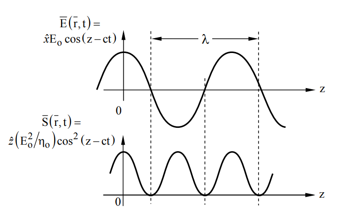
    \[ \overline{\mathrm{E}}(\overline{\mathrm{r}}, \mathrm{t})=\hat{x} \mathrm{E}_{\mathrm{o}} \cos (\mathrm{z}-\mathrm{ct}) \ [\mathrm{V} / \mathrm{m}]\]

    \[\overline{\mathrm{H}}(\overline{\mathrm{r}}, \mathrm{t})=\hat{y} \sqrt{\frac{\varepsilon_{\mathrm{o}}}{\mu_{\mathrm{o}}}} \mathrm{E}_{\mathrm{o}} \cos (\mathrm{z}-\mathrm{ct}) \ \left[\mathrm{A} / \mathrm{m}^{2}\right] \]

    The flux density for this wave is given by the Poynting overlinetor \(\overline S\)(t) (2.7.12):

    \[\overline{\mathrm{S}}(\mathrm{t})=\overline{\mathrm{E}} \times \overline{\mathrm{H}}=\hat{z} \frac{\mathrm{E}_{\mathrm{o}}^{2}}{\eta_{\mathrm{o}}} \cos ^{2}(\mathrm{z}-\mathrm{ct}) \ \left[\mathrm{W} / \mathrm{m}^{2}\right] \]

    where the characteristic impedance of free space is \(\eta_{0}=\sqrt{\mu_{0} / \varepsilon_{0}} \) ohms (2.2.19). The time average of \(\overline S\)(t) in (2.7.36) is \(\hat{z} \mathrm{E}_{\mathrm{o}}^{2} / 2 \eta_{\mathrm{o}} \ \left[\mathrm{W} / \mathrm{m}^{2}\right] \).

    The electric and magnetic energy densities for this wave can be found from (2.7.7–8):

    \[ \mathrm{W}_{\mathrm{e}}=\frac{1}{2} \varepsilon|\overline{\mathrm{E}}|^{2}=\frac{1}{2} \varepsilon_{0} \mathrm{E}_{0}^{2} \cos ^{2}(\mathrm{z}-\mathrm{ct})\left[\mathrm{J} / \mathrm{m}^{3}\right] \qquad\qquad\quad \text { (electric energy density) }\]

    \[\mathrm{W}_{\mathrm{m}}=\frac{1}{2} \mu|\overline{\mathrm{H}}|^{2}=\frac{1}{2} \varepsilon_{\mathrm{o}} \mathrm{E}_{\mathrm{o}}^{2} \cos ^{2}(\mathrm{z}-\mathrm{ct})\left[\mathrm{J} / \mathrm{m}^{3}\right] \qquad \qquad \quad(\text { magnetic energy density }) \]

    Note that these two energy densities, We and Wm, are equal, non-negative, and sinusoidal in behavior at twice the spatial frequency k = 2\(\pi\)/\(\lambda\) [radians/m] of the underlying wave, where cos2(z - ct) = 0.5[1 + cos 2(z - ct)], as illustrated in Figure 2.7.1; their frequency f[Hz] is also double that of the underlying wave. They have the same space/time form as the flux density, except with a different magnitude.

    The complex electric and magnetic fields corresponding to (2.7.34–5) are:

    \[\overline{\mathrm{\underline{E}}}(\overline{\mathrm{r}})=\hat{x} \mathrm{\underline{E}}_{\mathrm{o}} \ [\mathrm{V} / \mathrm{m}] \]

    \[\overline{\mathrm{\underline{H}}}(\overline{\mathrm{r}})=\hat{y} \sqrt{\varepsilon_{\mathrm{o}} / \mu_{\mathrm{o}}} \mathrm{\underline{E}}_{\mathrm{o}} \ \left[\mathrm{A} / \mathrm{m}^{2}\right] \]

    The real and imaginary parts of the complex power for this uniform plane wave indicate the time average and reactive powers, respectively:

    \[\langle\overline{\mathrm{S}}(\mathrm{t})\rangle=\frac{1}{2} \mathrm{R}_{\mathrm{e}}[\overline{\mathrm{\underline{S}}}]=\frac{1}{2} \mathrm{R}_{\mathrm{e}}\left[\overline{\mathrm{\underline{E}}} \times \overline{\mathrm{\underline{H}}}^{*}\right]=\hat{z} \frac{1}{2 \eta_{\mathrm{o}}}\left|\overline{\mathrm{\underline{E}}}_{\mathrm{o}}\right|^{2}=\hat{z} \frac{1}{2} \eta_{\mathrm{o}}\left|\overline{\mathrm{\underline{H}}}_{\mathrm{o}}\right|^{2} \ \left[\mathrm{W} / \mathrm{m}^{2}\right] \]

    \[ \mathrm{I}_{\mathrm{m}}\{\overline{\mathrm{\underline{S}}}(\overline{\mathrm{r}})\}=\mathrm{I}_{\mathrm{m}}\left\{\overline{\mathrm{\underline{E}}} \times \overline{\mathrm{\underline{H}}}^{*}\right\}=0\]

    If two superimposed plane waves are propagating in opposite directions with the same polarization, then the imaginary part of the Poynting overlinetor is usually non-zero. Positive reactive power flowing into a volume is generally associated with an excess of time-average magnetic energy storage over electric energy storage in that volume, and vice-versa, with negative reactive power input corresponding to excess electric energy storage.

    Figure 2.7.1.PNG
    Figure \(\PageIndex{1}\): Electric field, electric and magnetic storage, and wave intensity for a uniform plane wave.

    Example \(\PageIndex{B}\)

    Two equal x-polarized plane waves are propagating along the z axis in opposite directions such that \( \overline E \)(t) = 0 at z = 0 for all time t. What is \(\underline{\mathrm{\overline S}}(\mathrm{z})\)?

    Solution

    \(\overline{\mathrm{\underline{E}}}(\mathrm{z})=\hat{x} \mathrm{E}_{\mathrm{o}}\left(\mathrm{e}^{-\mathrm{jkz}}-\mathrm{e}^{+\mathrm{jkz}}\right)=0\) at z = 0; and \(\overline{\mathrm{\underline{H}}}(\mathrm{z})=\hat{y}\left(\mathrm{E}_{\mathrm{o}} / \mathrm{\eta}_{\mathrm{o}}\right)\left(\mathrm{e}^{-\mathrm{j} \mathrm{k} \mathrm{z}}+\mathrm{e}^{+\mathrm{j} \mathrm{k} \mathrm{z}}\right)\), so \(\overline{\underline{S}}=\overline{\underline{E}} \times \underline{\overline{H}}^{*}=\hat{z}\left(E_{\mathbf{o}}^{2} / \eta_{\mathbf{o}}\right)\left(\mathrm{e}^{-\mathrm{j} 2 \mathrm{k} \mathbf{z}}-\mathrm{e}^{+\mathrm{j} 2 \mathrm{k} \mathbf{z}}\right)=-\hat{z} 2 \mathrm{j}\left(\mathrm{E}_{\mathrm{o}}^{2} / \eta_{\mathrm{o}}\right) \sin (2 \mathrm{kz})\). \(\underline{\overline{S}}\) is pure imaginary and varies sinusoidally along z between inductive and capacitive reactive power, with nulls at intervals of \(\lambda\)/2.


    This page titled 2.7: Power and Energy in the Time and Frequency Domains and the Poynting Theorem is shared under a CC BY-NC-SA 4.0 license and was authored, remixed, and/or curated by David H. Staelin (MIT OpenCourseWare) via source content that was edited to the style and standards of the LibreTexts platform; a detailed edit history is available upon request.