
4.6: Flux tubes and field mapping
- Page ID
- 25004
\( \newcommand{\vecs}[1]{\overset { \scriptstyle \rightharpoonup} {\mathbf{#1}} } \)
\( \newcommand{\vecd}[1]{\overset{-\!-\!\rightharpoonup}{\vphantom{a}\smash {#1}}} \)
\( \newcommand{\dsum}{\displaystyle\sum\limits} \)
\( \newcommand{\dint}{\displaystyle\int\limits} \)
\( \newcommand{\dlim}{\displaystyle\lim\limits} \)
\( \newcommand{\id}{\mathrm{id}}\) \( \newcommand{\Span}{\mathrm{span}}\)
( \newcommand{\kernel}{\mathrm{null}\,}\) \( \newcommand{\range}{\mathrm{range}\,}\)
\( \newcommand{\RealPart}{\mathrm{Re}}\) \( \newcommand{\ImaginaryPart}{\mathrm{Im}}\)
\( \newcommand{\Argument}{\mathrm{Arg}}\) \( \newcommand{\norm}[1]{\| #1 \|}\)
\( \newcommand{\inner}[2]{\langle #1, #2 \rangle}\)
\( \newcommand{\Span}{\mathrm{span}}\)
\( \newcommand{\id}{\mathrm{id}}\)
\( \newcommand{\Span}{\mathrm{span}}\)
\( \newcommand{\kernel}{\mathrm{null}\,}\)
\( \newcommand{\range}{\mathrm{range}\,}\)
\( \newcommand{\RealPart}{\mathrm{Re}}\)
\( \newcommand{\ImaginaryPart}{\mathrm{Im}}\)
\( \newcommand{\Argument}{\mathrm{Arg}}\)
\( \newcommand{\norm}[1]{\| #1 \|}\)
\( \newcommand{\inner}[2]{\langle #1, #2 \rangle}\)
\( \newcommand{\Span}{\mathrm{span}}\) \( \newcommand{\AA}{\unicode[.8,0]{x212B}}\)
\( \newcommand{\vectorA}[1]{\vec{#1}} % arrow\)
\( \newcommand{\vectorAt}[1]{\vec{\text{#1}}} % arrow\)
\( \newcommand{\vectorB}[1]{\overset { \scriptstyle \rightharpoonup} {\mathbf{#1}} } \)
\( \newcommand{\vectorC}[1]{\textbf{#1}} \)
\( \newcommand{\vectorD}[1]{\overrightarrow{#1}} \)
\( \newcommand{\vectorDt}[1]{\overrightarrow{\text{#1}}} \)
\( \newcommand{\vectE}[1]{\overset{-\!-\!\rightharpoonup}{\vphantom{a}\smash{\mathbf {#1}}}} \)
\( \newcommand{\vecs}[1]{\overset { \scriptstyle \rightharpoonup} {\mathbf{#1}} } \)
\(\newcommand{\longvect}{\overrightarrow}\)
\( \newcommand{\vecd}[1]{\overset{-\!-\!\rightharpoonup}{\vphantom{a}\smash {#1}}} \)
\(\newcommand{\avec}{\mathbf a}\) \(\newcommand{\bvec}{\mathbf b}\) \(\newcommand{\cvec}{\mathbf c}\) \(\newcommand{\dvec}{\mathbf d}\) \(\newcommand{\dtil}{\widetilde{\mathbf d}}\) \(\newcommand{\evec}{\mathbf e}\) \(\newcommand{\fvec}{\mathbf f}\) \(\newcommand{\nvec}{\mathbf n}\) \(\newcommand{\pvec}{\mathbf p}\) \(\newcommand{\qvec}{\mathbf q}\) \(\newcommand{\svec}{\mathbf s}\) \(\newcommand{\tvec}{\mathbf t}\) \(\newcommand{\uvec}{\mathbf u}\) \(\newcommand{\vvec}{\mathbf v}\) \(\newcommand{\wvec}{\mathbf w}\) \(\newcommand{\xvec}{\mathbf x}\) \(\newcommand{\yvec}{\mathbf y}\) \(\newcommand{\zvec}{\mathbf z}\) \(\newcommand{\rvec}{\mathbf r}\) \(\newcommand{\mvec}{\mathbf m}\) \(\newcommand{\zerovec}{\mathbf 0}\) \(\newcommand{\onevec}{\mathbf 1}\) \(\newcommand{\real}{\mathbb R}\) \(\newcommand{\twovec}[2]{\left[\begin{array}{r}#1 \\ #2 \end{array}\right]}\) \(\newcommand{\ctwovec}[2]{\left[\begin{array}{c}#1 \\ #2 \end{array}\right]}\) \(\newcommand{\threevec}[3]{\left[\begin{array}{r}#1 \\ #2 \\ #3 \end{array}\right]}\) \(\newcommand{\cthreevec}[3]{\left[\begin{array}{c}#1 \\ #2 \\ #3 \end{array}\right]}\) \(\newcommand{\fourvec}[4]{\left[\begin{array}{r}#1 \\ #2 \\ #3 \\ #4 \end{array}\right]}\) \(\newcommand{\cfourvec}[4]{\left[\begin{array}{c}#1 \\ #2 \\ #3 \\ #4 \end{array}\right]}\) \(\newcommand{\fivevec}[5]{\left[\begin{array}{r}#1 \\ #2 \\ #3 \\ #4 \\ #5 \\ \end{array}\right]}\) \(\newcommand{\cfivevec}[5]{\left[\begin{array}{c}#1 \\ #2 \\ #3 \\ #4 \\ #5 \\ \end{array}\right]}\) \(\newcommand{\mattwo}[4]{\left[\begin{array}{rr}#1 \amp #2 \\ #3 \amp #4 \\ \end{array}\right]}\) \(\newcommand{\laspan}[1]{\text{Span}\{#1\}}\) \(\newcommand{\bcal}{\cal B}\) \(\newcommand{\ccal}{\cal C}\) \(\newcommand{\scal}{\cal S}\) \(\newcommand{\wcal}{\cal W}\) \(\newcommand{\ecal}{\cal E}\) \(\newcommand{\coords}[2]{\left\{#1\right\}_{#2}}\) \(\newcommand{\gray}[1]{\color{gray}{#1}}\) \(\newcommand{\lgray}[1]{\color{lightgray}{#1}}\) \(\newcommand{\rank}{\operatorname{rank}}\) \(\newcommand{\row}{\text{Row}}\) \(\newcommand{\col}{\text{Col}}\) \(\renewcommand{\row}{\text{Row}}\) \(\newcommand{\nul}{\text{Nul}}\) \(\newcommand{\var}{\text{Var}}\) \(\newcommand{\corr}{\text{corr}}\) \(\newcommand{\len}[1]{\left|#1\right|}\) \(\newcommand{\bbar}{\overline{\bvec}}\) \(\newcommand{\bhat}{\widehat{\bvec}}\) \(\newcommand{\bperp}{\bvec^\perp}\) \(\newcommand{\xhat}{\widehat{\xvec}}\) \(\newcommand{\vhat}{\widehat{\vvec}}\) \(\newcommand{\uhat}{\widehat{\uvec}}\) \(\newcommand{\what}{\widehat{\wvec}}\) \(\newcommand{\Sighat}{\widehat{\Sigma}}\) \(\newcommand{\lt}{<}\) \(\newcommand{\gt}{>}\) \(\newcommand{\amp}{&}\) \(\definecolor{fillinmathshade}{gray}{0.9}\)\(\newcommand{\oiiintD}{\mathop{
Static field flux tubes
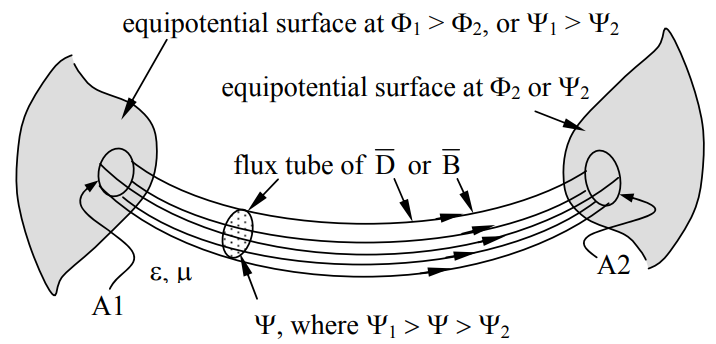
Flux tubes are arbitrarily designated bundles of static electric or magnetic field lines in charge free regions, as illustrated in Figure 4.6.1.
The divergence of such static fields is zero by virtue of Gauss’s laws, and their curl is zero by virtue of Faraday’s and Ampere’s laws. The integral forms of Gauss’s laws, (2.4.17) and (2.4.18), say that the total electric displacement D or magnetic flux B crossing the surface A of a volume V must be zero in a charge-free region:
\[ \oiint_{\mathrm{A}}(\overrightarrow{\mathrm{D}} \bullet \hat{n}) \mathrm{d} \mathrm{a}=0 \nonumber \]
\[\oiint_{\mathrm{A}}(\overrightarrow{\mathrm{B}} \bullet \hat{n}) \mathrm{d} \mathrm{a}=0 \nonumber \]
Therefore if the walls of flux tubes are parallel to the fields then the walls contribute nothing to the integrals (4.6.1) and (4.6.2) and the total flux entering the area A1 of the flux tube at one end (A1) must equal that exiting through the area A2 at the other end, as illustrated:
\[ \oiint_{\mathrm{A} 1}(\overrightarrow{\mathrm{D}} \bullet \hat{n}) \mathrm{d} \mathrm{a}=-\oiint_{\mathrm{A} 2}(\overrightarrow{\mathrm{D}} \bullet \hat{n}) \mathrm{d} \mathrm{a} \nonumber \]
\[ \oiint_{\mathrm{A} 1}(\overrightarrow{\mathrm{B}} \bullet \hat{n}) \mathrm{d} \mathrm{a}=-\oiint_{\mathrm{A} 2}(\overrightarrow{\mathrm{B}} \bullet \hat{n}) \mathrm{d} \mathrm{a} \nonumber \]
Consider two surfaces with potential differences between them, as illustrated in Figure 4.6.1. A representative flux tube is shown and all other fields are omitted from the figure. The field lines could correspond to either \(\overrightarrow{\mathrm{D}}\) or \(\overrightarrow{\mathrm{B}}\). Constant ε and μ are not required for \(\overrightarrow{\mathrm{D}}\) and \(\overrightarrow{\mathrm{B}}\) flux tubes because D and \(\overrightarrow{\mathrm{B}}\) already incorporate the effects of inhomogeneous media. If the permittivity ε and permeability μ were constant then the figure could also apply to \(\overrightarrow{\mathrm{E}}\) or \(\overrightarrow{\mathrm{H}}\), respectively.
Field mapping
\(\overrightarrow{\mathrm{E}}\) and \(\overrightarrow{\mathrm{H}}\) are gradients of the potentials Φ and Ψ, respectively [see (4.6.2) and (4.6.5)], and therefore the equipotential surfaces are perpendicular to their corresponding fields, as suggested in Figure 4.6.1. This orthogonality leads to a useful technique called field mapping for sketching approximately correct field distributions given arbitrarily shaped surfaces at known potentials. The method is particularly simple for “two-dimensional” geometries that depend only on the x,y coordinates and are independent of z, such as the pair of circular surfaces illustrated in Figure 4.6.2(a) and the pair of ovals in Figure 4.6.2(b). Assume that the potential of the inner surface is \(\Phi_{1}\) or \(\Psi_{1}\), and that at the outer surface is \(\Phi_{2}\) or \( \Psi_{2}\).
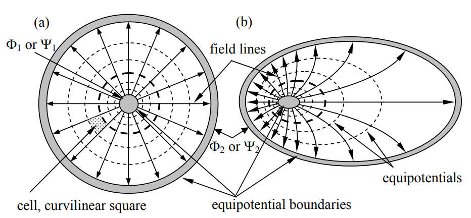
Because: 1) the lateral spacing between adjacent equipotential surfaces and (in two dimensional geometries) between adjacent field lines are both inversely proportional to the local field strength, and 2) the equipotentials and field lines are mutually orthogonal, it follows that the rectangular shape of the cells formed by these adjacent lines is preserved over the field even as the field strengths and cell sizes vary. That is, the curvilinear square illustrated in Figure 4.6.2(a) has approximately the same shape (but not size) as all other cells in the figure, and approaches a perfect square as the cells are subdivided indefinitely. If sketched perfectly, any two dimensional static potential distribution can be subdivided indefinitely into such curvilinear square cells.
One algorithm for performing such a subdivision is to begin by sketching a first-guess equipotential surface that: 1) separates the two (or more) equipotential boundaries and 2) is orthogonal to the first-guess field lines, which also can be sketched. These field lines must be othogonal to the equipotential boundaries. For example, this first sketched surface might have potential \(\left(\Phi_{1}+\Phi_{2}\right) / 2\), where \(\Phi_{1}\) and \(\Phi_{2}\) are the applied potentials. The spacing between the initially sketched field lines and between the initial equipotential surfaces should form approximate curvilinear squares. Each such square can then be subdivided into four smaller curvilinear squares using the same algorithm. If the initial guesses were correct, then the curvilinear squares approach true squares when infinitely subdivided. If they do not, the first guess is revised appropriately and the process can be repeated until the desired insight or perfection is achieved. In general there will be some fractional squares arranged along one of the field lines, but these become negligible in the limit.
Figure 4.6.2(a) illustrates how the flux tubes in a co-axial geometry are radial with field strength inversely proportional to radius. Therefore, when designing systems limited by the maximum allowable field strength, one avoids incorporating surfaces with small radii of curvature or sharp points. Figure 4.6.2(b) illustrates how the method can be adapted to arbitrarily shaped boundaries, albeit with more difficulty. Computer-based algorithms using relaxation techniques can implement such strategies rapidly for both two-dimensional and three dimensional geometries. In three dimensions, however, the spacing between field lines varies inversely with the square root of their strength, and so the height-to-width ratio of the curvilinear 3-dimensional rectangles formed by the field lines and potentials is not preserved across the structure.