
6.1: Force-induced electric and magnetic fields


- Last updated
- Jun 7, 2025
- Save as PDF

( \newcommand{\kernel}{\mathrm{null}\,}\)
Introduction
Chapter 5 explained how electric and magnetic fields could exert force on charges, currents, and media, and how electrical power into such devices could be transformed into mechanical power. Chapter 6 explores several types of practical motors and actuators built using these principles, where an actuator is typically a motor that throws a switch or performs some other brief task from time to time. Chapter 6 also explores the reverse transformation, where mechanical motion alters electric or magnetic fields and converts mechanical to electrical power. Absent losses, conversions to electrical power can be nearly perfect and find application in electrical generators and mechanical sensors.
Section 6.1.2 first explores how mechanical motion of conductors or charges through magnetic fields can generate voltages that can be tapped for power. Two charged objects can also be forcefully separated, lengthening the electric field lines connecting them and thereby increasing their voltage difference, where this increased voltage can be tapped for purposes of sensing or electrical power generation. Section 6.1.3 then shows in the context of a currentcarrying wire in a magnetic field how power conversion can occur in either direction.
Motion-induced voltages
Any conductor moving across magnetic field lines acquires an open-circuit voltage that follows directly from the Lorentz force law (6.1.1)18:
→f=q(→E+→v×μo→H)
Consider the electron illustrated in Figure 6.1.1, which has charge –e and velocity →v.
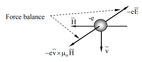
18 Some textbooks present alternative explanations that lead to the same results. The explanation here views matter as composed of charged particles governed electromagnetically solely by the Lorentz force law, and other forces, such as the Kelvin force densities acting on media discussed in Section 4.5, are derived from it.
It is moving perpendicular to →H and therefore experiences a Lorentz force on it of −e→v×μo→H. It experiences that force even inside a moving wire and will accelerate in response to it. This force causes all free electrons inside the conductor to move until the resulting surface charges produce an equilibrium electric field distribution such that the net force on any electron is zero.
In the case of a moving open-circuited wire, the free charges (electrons) will move inside the wire and accumulate toward its ends until there is sufficient electric potential across the wire to halt their movement everywhere. Specifically, this Lorentz force balance requires that the force −e→Ee on the electrons due to the resulting electric field →Ee be equal and opposite to those due to the magnetic field −e→v×μo→H, that is:
−eˉv×μ0ˉH=eˉEe
Therefore the equilibrium electric field inside the wire must be:
→Ee=−→v×μo→H
There should be no confusion about →Ee being non-zero inside a conductor. It is the net force on free electrons that must be zero in equilibrium, not the electric field →Ee. The electric Lorentz force q→Ee must balance the magnetic Lorentz force or otherwise the charges will experience a net force that continues to move them until there is such balance.
Figure 6.1.2 illustrates such a wire of length W moving at velocity →v perpendicular to →H.
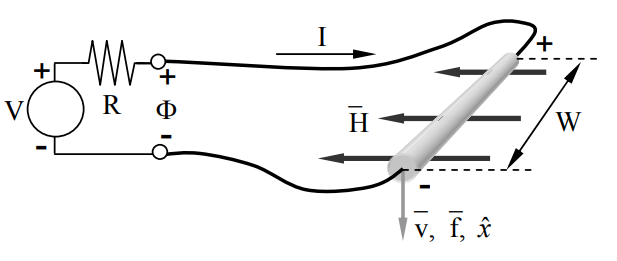
If the wire were open-circuited, the potential Φ across it would be the integral of the electric field necessary to cancel the magnetic forces on the electrons, where:
Φ=vμoHW
and the signs and directions are as indicated in the figure. We assume that the fields, wires, and velocity →v in the figure are all orthogonal so that →v×μo→H contributes no potential differences except along the wire of length W.
A large metal airplane flies at 300 m s-1 relative to a vertical terrestrial magnetic field of ~10-4 Teslas (1 gauss). What is the open-circuit voltage V wingtip to wingtip if the wingspan W is ~40 meters? If →B points upwards, is the right wing positive or negative?
Solution
The electric field induced inside the metal is −→v×μo→H (4.3.2), so the induced voltage V=WvμoH≅40×300×1.26×10−6×10−4≅1.5×10⁻⁶ volts, and the right wingtip is positive.
Induced currents and back voltages
If the moving wire of Figure 6.1.2 is connected to a load R, then current I will flow as governed by Ohm’s law. I depends on Φ, R, and the illustrated Thevenin voltage V:
I=(V−Φ)/R=(V−vμoHW)/R
The current can be positive or negative, depending on the relative values of V and the motioninduced voltage Φ. From (5.2.7) we see that the magnetic force density on the wire is →F=→I×μo→H [Nm−1]. The associated total force →fbe exerted on the wire by the environment and by →H follows from (6.1.5) and is:
→fbe=→I×μo→HW=ˆxμoHW(V−Φ)/R[N]
where the unit vector ˆx is parallel to →v.
Equation (6.1.6) enables us to compute the mechanical power delivered to the wire by the environment (Pbe) or, in the reverse direction, by the wire to the environment (Poe), where Pbe = - Poe. If the voltage source V is sufficiently great, then the system functions as a motor and the mechanical power Poe delivered to the environment by the wire is:
POe=ˉfoe∙→v=vμoHW(V−Φ)/R=Φ(V−Φ)/R[W]
The electrical power Pe delivered by the moving wire to the battery and resistor equals the mechanical power Pbe delivered to the wire by the environment, where I is given by (6.1.5):
Pe=−VI+I2R=−[V(V−Φ)/R]+[(V−Φ)2/R]=[(V−Φ)/R][−V+(V−Φ)]=−Φ(V−Φ)/R=Pbe[W]
The negative sign in the first term of (6.1.8) is associated with the direction of I defined in Figure 6.1.2; I flows out of the Thevenin circuit while Pe flows in. If V is zero, then the wire delivers maximum power, Φ2/R. As V increases, this delivered power diminishes and then becomes negative as the system ceases to be an electrical generator and becomes a motor. As a motor the mechanical power delivered to the wire by the environment becomes negative, and the electrical power delivered by the Thevenin source becomes positive. That is, we have a:
Motor:If mechanical power out Poe>0, V>Φ=vμoHW, or v<V/μoHW
Generator:If electrical power out Pe>0,V<Φ, or v>V/μoHW
We call Φ the “back voltage” of a motor; it increases as the motor velocity v increases until it equals the voltage V of the power source and Pe = 0. If the velocity increases further so that Φ > V, the motor becomes a generator. When V = Φ, then I = 0 and the motor moves freely without any electromagnetic forces.
This basic coupling mechanism between magnetic and mechanical forces and powers can be utilized in many configurations, as discussed further below.
A straight wire is drawn at velocity v=ˆx10 m s−1 between the poles of a 0.1-Tesla magnet; the velocity vector, wire direction, and field direction are all orthogonal to each other. The wire is externally connected to a resistor R = 10-5 ohms. What mechanical force →f is exerted on the wire by the magnetic field →B? The geometry is illustrated in Figure 6.1.2.
Solution
The force exerted on the wire by its magnetic environment (6.1.6) is →fbe=→I×→HμoW [N], where the induced current I = -Φ/R and the back voltage Φ = vμoHW [V]. Therefore:
fbe=−ˆxμoHWΦ/R=−ˆxv(μoHW)2/R=−ˆx10×(0.1×0.1)2/10−5=1 [N],
opposite to →v.