
6.4: Linear magnetic motors and actuators


- Last updated
- Jun 7, 2025
- Save as PDF

( \newcommand{\kernel}{\mathrm{null}\,}\)
Solenoid Actuators
Compact actuators that flip latches or switches, increment a positioner, or impact a target are often implemented using solenoids. Solenoid actuators are usually cylindrical coils with a slideably disposed high-permeability cylindrical core that is partially inserted at rest, and is drawn into the solenoid when current flows, as illustrated in Figure 6.4.1. A spring (not illustrated) often holds the core near its partially inserted rest position.
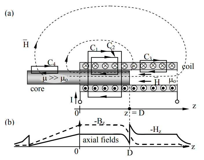
If we assume the diameter of the solenoid is small compared to its length, then the fringing fields at the ends of the coil and core can be neglected relative to the field energy stored elsewhere along the solenoid. If we integrate →H along contour C1 (see figure) we obtain zero from Ampere’s law because no net current flows through C1 and ∂→D/∂t≅0:
∮C→H∙d→s=⊂⊃∬A(→J+∂→D/∂t)∙ˆnda=0
This implies →H≅0 outside the solenoid unless Hz is approximately uniform outside, a possibility that is energetically disfavored relative to H being purely internal to the coil. Direct evaluation of →H using the Biot-Savart law (1.4.6) also yields →H≅0 outside. If we integrate →H along contour C2, which passes along the axis of the solenoid for unit distance, we obtain:
∮C2→H∙d→s=NoI=−Hz
where No is defined as the number of turns of wire per meter of solenoid length. We obtain the same answer (6.4.2) regardless of the permeability along the contour C2, provided we are not near the ends of the solenoid or its moveable core. For example, (6.4.2) also applies to contour C3, while the integral of →H around C4 is zero because the encircled current there is zero.
Since (6.4.2) requires that Hz along the solenoid axis be approximately constant, Bz must be a factor of μ/μo greater in the permeable core than it is in the air-filled portions of the solenoid. Because boundary conditions require →B⊥ to be continuous at the core-air boundary, →H⊥ must be discontinuous there so that μHμ=μoHo, where Hμ and Ho are the axial values of H in the core and air, respectively. This appears to conflict with (6.4.2), which suggests →H inside the solenoid is independent of μ, but this applies only if we neglect fringing fields at the ends of the solenoid or near boundaries where μ changes. Thus the axial H varies approximately as suggested in Figure 6.4.1(b): it has a discontinuity at the boundary that relaxes toward constant H = NoI away from the boundary over a distance comparable to the solenoid diameter. Two representative field lines in Figure 6.4.1(a) suggest how →B diverges strongly at the end of the magnetic core within the solenoid while other field lines remain roughly constant until they diverge at the right end of the solenoid. The transition region between the two values of Bz at the end of the solenoid occurs over a distance roughly equal to the solenoid diameter, as suggested in Figure 6.4.1(b). The magnetic field lines →B and →H "repel" each other along the protruding end of the high permeability core on the left side of the figure, resulting in a nearly linear decline in magnetic field within the core there; at the left end of the core there is again a discontinuity in |Hz| because →B⊥ must be continuous.
Having approximated the field distribution we can now calculate energies and forces using the expression for magnetic energy density, Wm = μH2/2 [J m-3]. Except in the negligible fringing field regions at the ends of the solenoid and at the ends of its core, |H| ≅ NoI (6.4.2) and μH2 >> μoH2, so to simplify the solution we neglect the energy stored in air as we compute the magnetic force fz pulling on the core in the +z direction:
fz=−dwT/dz [N]
The energy in the core is confined largely to the length z within the solenoid, which has a crosssectional area A [m2]. The total magnetic energy wm thus approximates:
wm≅AzμH2/2 [J]
If we assume wT = wm and differentiate (6.4.4) assuming H is independent of z, we find the magnetic force expels the core from the solenoid, the reverse of the truth. To obtain the correct answer we must differentiate the total energy wT in the system, which includes any energy in the power source supplying the current I. To avoid considering a power supply we may alternatively assume the coil is short-circuited and carrying the same I as before. Since the instantaneous force on the core depends on the instantaneous I and is the same whether it is short-circuited or connected to a power source, we may set:
v=0=dΛ/dt
where:
Λ≅Nψm=N∬Aμ→Hμ∙d→a=NozμHμA
Hμ is the value of H inside the core (μ) and Noz is the number of turns of wire circling the core, where No is the number of turns per meter of coil length. But Hμ = Js [A m-1] = NoI, so:
Λ=N2oIzμA
I=Λ/(N2ozμA)
We now can compute wT using only wm because we have replaced the power source with a short circuit that stores no energy:
wT≅μH2μAz/2=μ(NoI)2Az/2=μ(Λ/μNoAz)2Az/2=Λ2/(μN2oAz2)
So (6.4.9) and (6.4.6) yield the force pulling the core into the solenoid:
fz=−dwTdz=−ddz[Λ2μN2o2Az]=(Λ/Noz)22Aμ=μH2μA2 [N]
where Hμ = H. This force is exactly the area A of the end of the core times the same magnetic pressure μH2/2 [Nm-2] we saw in (6.3.25), but this time the magnetic field is pulling on the core in the direction of the magnetic field lines, whereas before the magnetic field was pushing perpendicular to the field lines. This pressure equals the magnetic energy density Wm, as before. A slight correction for the non-zero influence of μo and associated small pressure from the air side could be made here, but more exact answers to this problem generally also require consideration of the fringing fields and use of computer tools.
It is interesting to note how electric and magnetic pressure [N/m2] approximates the energy density [J m-3] stored in the fields, where we have neglected the pressures applied from the lowfield side of the boundary when ε >> εo or μ >> μo. We have now seen examples where →E and →H both push or pull on boundaries from the high-field (usually air) side of a boundary, where both →E and →H pull in the direction of their field lines, and push perpendicular to them.
MEMS magnetic actuators
One form of magnetic MEMS switch is illustrated in Figure 6.4.2. A control current I2 deflects a beam carrying current I1. When the beam is pulled down toward the substrate, the switch (not shown) will close, and when the beam is repelled upward the switch will open. The Lorentz force law (1.2.1) states that the magnetic force →f on a charge q is q→v×μo→H, and therefore the force density per unit length →F [N m-1] on a current →I1=Nq→v induced by the magnetic field →H12 at position 1 produced by I2 is:
→F=Nq→v×μo→H12=→I1×μo→H12 [Nm−1]
N is the number of moving charges per meter of conductor length, and we assume that all forces on these charges are conveyed directly to the body of the conductor.
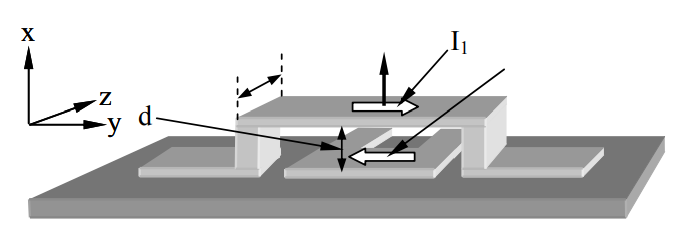
If the plate separation d << W, then fringing fields can be neglected and the I2-induced magnetic field affecting current I1 is →H12, which can be found from Ampere’s law (1.4.1) computed for a contour C circling I2 in a right-hand sense:
∮C→H∙d→s≅H122W=⊂⊃∬A→J∙ˆnda=I2
Thus →H12≅ˆzI2/2W. The upward pressure on the upper beam found from (6.4.11) and (6.4.12) is then:
→P=→F/W≅ˆxμoIlI2/2W2 [Nm−2]
If I1 = -I2 then the magnetic field between the two closely spaced currents is Ho′ = I1/W and (6.4.13) becomes →p=ˆxμoH′2o/2 [N m-2]; this expression for magnetic pressure is derived differently in (6.4.15).
This pressure on the top is downward if both currents flow in the same direction, upward if they are opposite, and zero if either is zero. This device therefore can perform a variety of logic functions. For example, if a switch is arranged so its contacts are closed in state “1” when the beam is forced upward by both I1 and I2 being positive (these currents were defined in the figure as flowing in opposite directions), and not otherwise, this is an “and” gate.
An alternate way to derive magnetic pressure (6.4.13) is to note that if the two currents I1 and I2 are anti-parallel, equal, and close together (d << W), then →H=0 outside the two conductors and Ho' is doubled in the gap between them so WHo' = I1. That is, if the integration contour C circles either current alone then (6.4.12) becomes:
∮C→H∙d→s≅H′oW=⊂⊃∬A→J∙ˆnda=I1=I2
But not all electrons comprising these currents see the same magnetic field because the currents closer to the two innermost conductor surfaces screen the outer currents, causing the magnetic field to approach zero inside the conductors, as suggested in Figure 6.4.3.
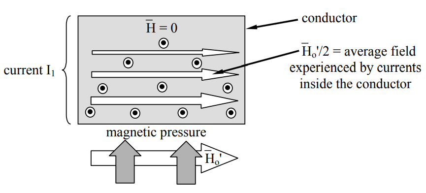
Therefore the average moving electron sees a magnetic field Ho'/2, half that at the surface28. Thus the total magnetic pressure upward on the upper beam given by (6.4.13) and (6.4.14) is:
→P=→F/W=→I1×μo→H′o/2W=ˆx(H′oW)(μoH′o/2W)=ˆxμoH′2o/2 [Nm−2](magnetic pressure)
where Ho' is the total magnetic field magnitude between the two conductors, and there is no magnetic field on the top of the upper beam to press in the opposite direction. This magnetic pressure [N m-2] equals the magnetic energy density [J m-3] stored in the magnetic field adjacent to the conductor (2.7.8).
28 A simple integral of the form used in (5.2.4) yields this same result for pressure.