9.3: Waves Guided within Cartesian Boundaries

Parallel-plate waveguides

We have seen in Section 9.2 that waves can be reflected at planar interfaces. For example, (9.2.14) and (9.2.16) describe the electric fields for a TE wave reflected from a planar interface at x = 0, and are repeated here:

\[\overline{\mathrm{\underline E}}_{\mathrm{i}}=\hat{y} \underline{\mathrm{E}}_{0} \mathrm{e}^{\mathrm{j} \mathrm{k}_{\mathrm{x}} \mathrm{x}-\mathrm{j} \mathrm{k}_{\mathrm{z}} \mathrm{z}} \ \left[\mathrm{V} \mathrm{m}^{-1}\right] \qquad \qquad \qquad \text{(incident TE wave)}\]

\[\overline{\mathrm{\underline E}}_{\mathrm{r}}=\hat{y} \underline{\mathrm{E}}_{\mathrm{r}}-\mathrm{jk}_{\mathrm{x}} \mathrm{x}-\mathrm{jk}_{\mathrm{z}} \mathrm{z} \qquad \qquad \qquad \text{(reflected TE wave) }\]

Note that the subscripts i and r denote “incident” and “reflected”, not “imaginary” and “real”. These equations satisfy the phase-matching boundary condition that \( \mathrm{k}_{\mathrm{z}}=\mathrm{k}_{\mathrm{zi}}=\mathrm{k}_{\mathrm{zr}}\). Therefore \( \left|\mathrm{k}_{\mathrm{x}}\right|\) is the same for the incident and reflected waves because for both waves \( \mathrm{k}_{\mathrm{x}}^{2}+\mathrm{k}_{\mathrm{z}}^{2}=\omega^{2} \mu \varepsilon\).

If the planar interface at x = 0 is a perfect conductor, then the total electric field there parallel to the conductor must be zero, implying \(\mathrm{\underline{E}_{r}=-\underline{E}_{0}} \). The superposition of these two incident and reflected waves is:

\[\overline{\mathrm{\underline E}}(\mathrm{x}, \mathrm{z})=\hat{y} \underline{\mathrm{E}}_{\mathrm{o}}\left(\mathrm{e}^{\mathrm{jk}_{\mathrm{x}} \mathrm{x}}-\mathrm{e}^{-\mathrm{j} \mathrm{k}_{\mathrm{x}} \mathrm{x}}\right) \mathrm{e}^{-\mathrm{j} \mathrm{k}_{\mathrm{z}} \mathrm{z}}=\hat{y} 2 \mathrm{j} \mathrm{\underline E}_{\mathrm{o}} \sin \mathrm{k}_{\mathrm{x}} \mathrm{xe}^{-\mathrm{j} \mathrm{k}_{\mathrm{z}} \mathrm{z}}\]

Thus \( \overline{\mathrm{E}}=0\) in a series of parallel planes located at x = d, where:

\[\mathrm{k}_{\mathrm{x}} \mathrm{d}=\mathrm{n} \pi \text { for } \mathrm{n}=0,1,2, \ldots \qquad \qquad \qquad \text{(guidance condition) }\]

Because \( \mathrm{k}_{\mathrm{x}}=2 \pi / \lambda_{\mathrm{x}}\), these planes of electric-field nulls are located at \( \mathrm{x}_{\text {nulls }}=\mathrm{n} \lambda_{\mathrm{x}} / 2\). A second perfect conductor could be inserted at any one of these x planes so that the waves would reflect back and forth and propagate together in the +z direction, trapped between the two conducting planes.

We can easily confirm that the boundary conditions are satisfied for the corresponding magnetic field \( \overline{\mathrm{H}}(\mathrm{x}, \mathrm{z})\) by using Faraday’s law:

\[ \overline{\mathrm{\underline H}}(\mathrm{x}, \mathrm{z})=-(\nabla \times \overline{\mathrm{\underline E}}) / \mathrm{j} \omega \mu=-\left(2 \mathrm{\underline E}_{\mathrm{o}} / \omega \mu\right)\left(\hat{x} \ \mathrm{jk}_{\mathrm{z}} \sin \mathrm{k}_{\mathrm{x}} \mathrm{x}+\hat{z} \ \mathrm{k}_{\mathrm{x}} \cos \mathrm{k}_{\mathrm{x}} \mathrm{x}\right) \mathrm{e}^{-\mathrm{j} \mathrm{k}_{\mathrm{z}} \mathrm{z}}\]

At \( \) we find \( \), , so this solution is valid.

Equation (9.3.4), \(\mathrm{k}_{\mathrm{x}} \mathrm{d}=\mathrm{n} \pi \ (\mathrm{n}=1,2, \ldots) \), is the guidance condition for parallel-plate waveguides that relates mode number to waveguide dimensions; d is the separation of the parallel plates. We can use this guidance condition to make the expressions (9.3.3) and (9.3.5) for \(\overline{\underline{\mathrm{E}}} \) and \(\overline{\underline{\mathrm{H}}} \) more explicit by replacing k_xx with n\(\pi\)x/d, and k_z with \(2 \pi / \lambda_{\mathrm{z}}\):

\[\overline{\mathrm{\underline E}}(\mathrm{x}, \mathrm{z})=\hat{y} 2 \mathrm{j} \mathrm{\underline E}_{\mathrm{o}} \sin \left(\frac{\mathrm{n} \pi \mathrm{x}}{\mathrm{d}}\right) \mathrm{e}^{-\frac{\mathrm{j} 2 \pi \mathrm{z}}{\lambda_{\mathrm{z}}}} \qquad\qquad\qquad\left(\overline{\mathrm{E}} \text { for } \mathrm{TE}_{\mathrm{n}} \text { mode }\right)\]

\[\overline{\mathrm{\underline H}}(\mathrm{x}, \mathrm{z})=-\frac{2 \mathrm{E}_{\mathrm{o}}}{\omega \mu}\left[\hat{x} \mathrm{j} \frac{2 \pi}{\lambda_{\mathrm{z}}} \sin \left(\frac{\mathrm{n} \pi \mathrm{x}}{\mathrm{d}}\right)+\hat{z} \frac{\mathrm{n} \pi}{\mathrm{d}} \cos \left(\frac{\mathrm{n} \pi \mathrm{x}}{\mathrm{d}}\right)\right] \mathrm{e}^{-\frac{\mathrm{j} 2 \pi \mathrm{z}}{\lambda_{\mathrm{z}}}}\]

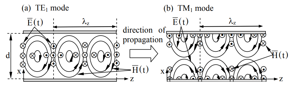
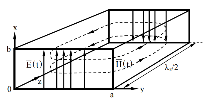
These electric and magnetic fields correspond to a waveguide mode propagating in the +z direction, as illustrated in Figure 9.3.1(a) for a waveguide with plates separated by distance d.

The direction of propagation can be inferred from the Poynting vector \(\overline{\mathrm{\underline S}}=\overline{\mathrm{\underline E}} \times \overline{\mathrm{\underline H}}^{*} \). Because this is a TE wave and there is only one half wavelength between the two conducting plates (n = 1), this is designated the TE₁ mode of a parallel-plate waveguide. Because Maxwell’s equations are linear, several propagating modes with different values of n can be active simultaneously and be superimposed.

These fields are periodic in both the x and z directions. The wavelength \( \lambda_{\mathrm{z}}\) along the z axis is called the waveguide wavelength and is easily found using \(\mathrm{k}_{\mathrm{z}}=2 \pi / \lambda_{\mathrm{z}}\) where \( \mathrm{k^{2}=k_{x}^{2}+k_{z}^{2}}=\omega^{2} \mu \varepsilon\):

\[\lambda_{\mathrm{z}}=2 \pi\left(\mathrm{k}^{2}-\mathrm{k}_{\mathrm{x}}^{2}\right)^{-0.5}=2 \pi\left[(\omega / \mathrm{c})^{2}-(\mathrm{n} \pi / \mathrm{d})^{2}\right]^{-0.5} \qquad\qquad\qquad \text { (waveguide wavelength) }\]

Figure \(\PageIndex{1}\): TE₁ and TM₁ modes of parallel-plate waveguides.

Only those TE_n modes having \(\mathrm{n}<\omega \mathrm{d} / \mathrm{c} \pi=2 \mathrm{d} / \lambda\) have non-imaginary waveguide wavelengths \( \) and propagate. Propagation ceases when the mode number n increases to the point where \(\mathrm{n} \pi / \mathrm{d} \geq \mathrm{k} \equiv 2 \pi / \lambda \equiv \omega / \mathrm{c}\). This propagation requirement can also be expressed in terms of a minimum frequency ω of propagation, or cut-off frequency, for any TE mode:

\[\omega_{\mathrm{TEn}}=\mathrm{n} \pi \mathrm{c} / \mathrm{d} \qquad \qquad \qquad \text{(cut-off frequency for } \mathrm{TE_n} \text{ mode) }\]

Thus each TE_n mode has a minimum frequency ω_TEn for which it can propagate, as illustrated in Figure 9.3.2.

Figure \(\PageIndex{2}\): Propagation frequencies of TE_n modes in parallel-plate waveguides.

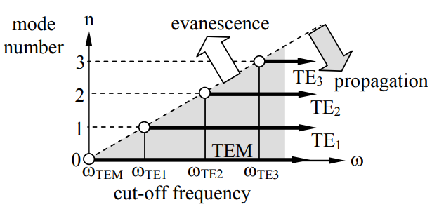
The TE₀ mode has zero fields everywhere and therefore does not exist. The TM₀ mode can propagate even DC signals, but is identical to the TEM mode. This same relationship can also be expressed in terms of the maximum free-space wavelength \(\lambda_{\mathrm{TEn}}\) that can propagate:

\[\lambda_{\mathrm{TE}_{\mathrm{n}}}=2 \mathrm{d} / \mathrm{n} \qquad \qquad \qquad \text{(cut-off wavelength } \lambda_\mathrm{TE_n} \text{ for } \mathrm{TE_n} \text{ mode)}\]

For a non-TEM wave the longest free-space wavelength λ that can propagate in a parallel-plate waveguide of width d is 2d/n.

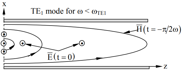
If ω < ω_TEn, then we have an evanescent wave; k_z, (9.3.6), and (9.3.7) become:

\[\mathrm{k}_{\mathrm{Z}}^{2}=\omega^{2} \mu \varepsilon-\mathrm{k}_{\mathrm{x}}^{2}<0, \ \underline{\mathrm{k}}_{\mathrm{Z}}=\pm \mathrm{j} \alpha\]

\[\overline{\mathrm{\underline E}}(\mathrm{x}, \mathrm{z})=\hat{y} 2 \mathrm{j} \mathrm{\underline E}_{\mathrm{o}} \sin (\mathrm{n} \pi \mathrm{x} / \mathrm{d}) \mathrm{e}^{-\alpha \mathrm{z}} \qquad\qquad\qquad\left(\overline{\mathrm{\underline E}} \text { for } \mathrm{TE}_{\mathrm{n}} \operatorname{mode}, \ \omega<\mathrm{T} \mathrm{En}\right)\]

\[\overline{\mathrm{\underline H}}(\mathrm{x}, \mathrm{z})=-(\nabla \times \overline{\mathrm{\underline E}}) / \mathrm{j} \omega \mu=-\left(2 \mathrm{\underline E}_{\mathrm{o}} / \omega \mu\right)\left(\hat{x} \alpha \sin \mathrm{k}_{\mathrm{x}} \mathrm{x}+\hat{z} \mathrm{k}_{\mathrm{x}} \cos \mathrm{k}_{\mathrm{x}} \mathrm{x}\right) \mathrm{e}^{-\alpha \mathrm{z}}\]

Such evanescent waves propagate no time average power, i.e., \( \mathrm{R}_{\mathrm{e}}\left\{\overline{\mathrm{S}}_{\mathrm{z}}\right\}=0\), because the electric and magnetic fields are 90 degrees out of phase everywhere and decay exponentially toward zero as z increases, as illustrated in Figure 9.3.3.

Figure \(\PageIndex{3}\): Evanescent TE₁ mode in a parallel-plate waveguide.

If we reflect a TM wave from a perfect conductor there again will be planar loci where additional perfectly conducting plates could be placed without violating boundary conditions, as suggested in Figure 9.3.1(b) for the TM₁ mode. Note that the field configuration is the same as for the TE₁ mode, except that \(\overline{\mathrm{E}}\) and \(\overline{\mathrm{H}}\) have been interchanged (allowed by duality) and phase shifted in the lateral direction to match boundary conditions. Between the plates the TE and TM field solutions are dual, as discussed in Section 9.2.6. Also note that TEM = TM₀₁.

Evaluation of Poynting’s vector reveals that the waves in Figure 9.3.1 are propagating to the right. If this waveguide mode were superimposed with an equal-strength wave traveling to the left, the resulting field pattern would be similar, but the magnetic and electric field distributions \(\overline{\mathrm{E}}(\mathrm{t})\) and \(\overline{\mathrm{H}}(\mathrm{t})\) would be shifted relative to one another by \(\lambda_{2} / 4\) along the z axis, and they would be 90o out of phase in time; the time-average power flow would be zero, and the reactive power \(\mathrm{I}_{\mathrm{m}}\{\overline{\mathrm{S}}\}\) would alternate between inductive (+j) and capacitive (-j) at intervals of \(\lambda_{\mathrm z} / 2 \) down the waveguide.

Because k_z/ω is frequency dependent, the shapes of waveforms evolve as they propagate. If the signal is narrowband, this evolution can be characterized simply by noting that the envelope of the waveform propagates at the “group velocity” v_g, and the modulated sinusoidal wave inside the envelope propagates at the “phase velocity” v_p, as discussed more fully in Section 9.5.2. These velocities are easily found from k(ω): v_p = ω/k and \(\mathrm{v}_{\mathrm{g}}=(\partial \mathrm{k} / \partial \omega)^{-1}\).

Figure \(\PageIndex{4}\): Dispersion relation and v_p and v_g for a parallel-plate waveguide.

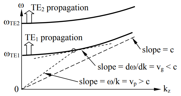
The phase and group velocities of waves in parallel-plate waveguides do not equal c, as can be deduced the dispersion relation plotted in Figure 9.3.4:

\[\mathrm{k}_{\mathrm{Z}}^{2}=\omega^{2} \mu \varepsilon-\mathrm{k}_{\mathrm{x}}^{2}=\omega^{2} / \mathrm{c}^{2}-(\mathrm{n} \pi / \mathrm{d})^{2} \qquad\qquad\qquad \text { (waveguide dispersion relation) }\]

The phase velocity v_p of a wave, which is the velocity at which the field distribution pictured in Figure 9.3.1 moves to the right, equals ω/k, which approaches infinity as ω approaches the cut-off frequency ω_TEn from above. The group velocity v_g, which is the velocity of energy or information propagation, equals dω/dk, which is the local slope of the dispersion relation ω(k) and can never exceed c. Both v_p and v_g approach \(c=(\mu \varepsilon)^{-0.5}\) as ω → ∞.

Example \(\PageIndex{A}\)

A TM₂ mode is propagating in the +z direction in a parallel-plate waveguide with plate separation d and free-space wavelength λ_o. What are \(\overline{\mathrm{\underline E}}\) and \(\overline{\mathrm{\underline H}}\)? What is λ_z? What is the decay length \(\alpha_{\mathrm{Z}}^{-1}\) when the mode is evanescent and \(\lambda_{\mathrm{o}}=2 \lambda_{\text {cut off }}\)?

Solution

We can superimpose incident and reflected TM waves or use duality to yield \(\overline{\mathrm{H}}(\mathrm{x}, \mathrm{y}) =\hat{y} \mathrm{H}_{0} \operatorname{cosk}_{\mathrm{x}} \mathrm{x} \ \mathrm{e}^{-\mathrm{jk}_{\mathrm{z}} \mathrm{z}}\), analogous to (9.3.3), where \(\mathrm{k}_{\mathrm{x}} \mathrm{d}=2 \pi\) for the TM₂ mode. Therefore \(\mathrm{k}_{\mathrm{x}}=2 \pi / \mathrm{d}\) and \(\mathrm{k}_{\mathrm{z}}=2 \pi / \lambda_{\mathrm{z}}=\left(\mathrm{k}_{\mathrm{o}}^{2}-\mathrm{k}_{\mathrm{x}}^{2}\right)^{0.5}=\left[\left(2 \pi / \lambda_{\mathrm{o}}\right)^{2}-(2 \pi / \mathrm{d})^{2}\right]^{0.5}\). Ampere’s law yields:

\[\begin{aligned}\overline{\mathrm{E}} &=\nabla \times \overline{\mathrm{\underline H}} / \mathrm{j} \omega \varepsilon=\left(\hat{x} \partial \mathrm{H}_{\mathrm{y}} / \partial \mathrm{z}+\hat{z} \mathrm{H}_{\mathrm{y}} / \partial \mathrm{x}\right) / \mathrm{j} \omega \varepsilon \\&=\left(\hat{x} \mathrm{k}_{\mathrm{z}} \cos \mathrm{k}_{\mathrm{x}} \mathrm{x}+\hat{z} \mathrm{jk}_{\mathrm{x}} \sin \mathrm{k}_{\mathrm{x}} \mathrm{x}\right)\left(\mathrm{H}_{\mathrm{o}} / \omega \varepsilon\right) \mathrm{e}^{-\mathrm{j} \mathrm{k}_{\mathrm{z}} \mathrm{z}}\end{aligned}\]

The waveguide wavelength \(\lambda_{\mathrm{z}}=2 \pi / \mathrm{k}_{\mathrm{z}}=\left(\lambda_{\mathrm{o}}^{-2}-\mathrm{d}^{-2}\right)^{0.5}\). Cutoff occurs when k_z = 0 , or \(\mathrm{k}_{\mathrm{o}}=\mathrm{k}_{\mathrm{x}}=2 \pi / \mathrm{d}=2 \pi / \lambda_{\mathrm{cut} \text { off }}\). Therefore \(\lambda_{\mathrm{o}}=2 \lambda_{\text {cut off }} \Rightarrow \lambda_{\mathrm{o}}=2 \mathrm{d}\), and \(\alpha_{0}^{-1}=\mathrm{\left(-j k_{z}\right)=\left(k_{x}^{2}\right. \left.-k_{0}^{2}\right)^{0.5}=\left[d^{-2}-(2 d)^{-2}\right]^{-0.5} / 2 \pi=d /\left(3^{0.5} \pi\right) \ [m]}\).

Rectangular waveguides

Waves can be trapped within conducting cylinders and propagate along their axis, rectangular and cylindrical waveguides being the most common examples. Consider the rectangular waveguide illustrated in Figure 9.3.5. The fields inside it must satisfy the wave equation:

\[\left(\nabla^{2}+\omega^{2} \mu \varepsilon\right) \overline{\mathrm{\underline E}}=0 \qquad \qquad\left(\nabla^{2}+\omega^{2} \mu \varepsilon\right) \overline{\mathrm{\underline H}}=0\]

where \(\nabla^{2} \equiv \partial^{2} / \partial x^{2}+\partial^{2} / \partial y^{2}+\partial^{2} / \partial z^{2}\).

Figure \(\PageIndex{5}\): Dominant mode in rectangular waveguide (TE₁₀).

Since the wave equation requires that the second spatial derivative of \(\overline{\mathrm{\underline E}}\) or \(\overline{\mathrm{\underline H}}\) equal \(\overline{\mathrm{\underline E}}\) or \(\overline{\mathrm{\underline H}}\) times a constant, these fields must be products of sinusoids or exponentials along each of the three cartesian coordinates, or sums of such products. For example, the wave equation and boundary conditions (\(\overline{\mathrm{E}}_{/ /}=0\) at x = 0 and y = 0) are satisfied by:

\[\mathrm{E}_{\mathrm{x}}=\sin \mathrm{k}_{\mathrm{y}} \mathrm{y}\left(\mathrm{A} \sin \mathrm{k}_{\mathrm{x}} \mathrm{x}+\mathrm{B} \cos \mathrm{k}_{\mathrm{x}} \mathrm{x}\right) \mathrm{e}^{-\mathrm{j} \mathrm{k}_{\mathrm{z}} \mathrm{z}}\]

\[\mathrm{E}_{\mathrm{y}}=\sin \mathrm{k}_{\mathrm{x}} \mathrm{x}\left(\mathrm{C} \sin \mathrm{k}_{\mathrm{y}} \mathrm{y}+\mathrm{D} \cos \mathrm{k}_{\mathrm{y}} \mathrm{y}\right) \mathrm{e}^{-\mathrm{j} \mathrm{k}_{\mathrm{z}} \mathrm{z}}\]

provided that the usual dispersion relation for uniform media is satisfied:

\[\mathrm{k}_{\mathrm{x}}^{2}+\mathrm{k}_{\mathrm{y}}^{2}+\mathrm{k}_{\mathrm{z}}^{2}=\mathrm{k}_{\mathrm{o}}^{2}=\omega^{2} \mu \varepsilon \qquad \qquad \qquad \text{(dispersion relation) }\]

These field components must also satisfy the boundary condition \(\overline{\mathrm{E}} _{/ /}=0 \) for x = b and y = a, which leads to the guidance conditions:

\[ \mathrm{k}_{\mathrm{x}} \mathrm{b}=\mathrm{n} \pi\]

\[\mathrm{k}_{\mathrm{y}} \mathrm{a}=\mathrm{m} \pi \qquad \qquad \qquad \text{(guidance conditions) }\]

We can already compute the cut-off frequency of propagation ω_mn for each mode, assuming our conjectured solutions are valid, as shown below. Cut-off occurs when a mode becomes evanescent, i.e., when \(\mathrm{k}_{\mathrm{o}}^{2}\) equals zero or becomes negative. At cut-off for the m,n mode:

\[\omega_{\mathrm{mn}} \mu \varepsilon=\mathrm{k}_{\mathrm{y}}^{2}+\mathrm{k}_{\mathrm{x}}^{2}=(\mathrm{m} \pi / \mathrm{a})^{2}+(\mathrm{n} \pi / \mathrm{b})^{2}\]

\[\omega_{\mathrm{mn}}=\left[(\mathrm{m} \pi \mathrm{c} / \mathrm{a})^{2}+(\mathrm{n} \pi \mathrm{c} / \mathrm{b})^{2}\right]^{0.5} \qquad \qquad \qquad \text { (cut-off frequencies) }\]

Since a ≥ b by definition, and the 0,0 mode cannot have non-zero fields, as shown later, the lowest frequency that can propagate is:

\[\omega_{10}=\pi \mathrm{c} / \mathrm{a}\]

which implies that the longest wavelength that can propagate in rectangular waveguide is \(\lambda_{\max }=2 \pi \mathrm{c} / \omega_{10}=2 \mathrm{a} \). If a > 2b, the second lowest cut-off frequency is ω₂₀ = 2ω₁₀, so such waveguides can propagate only a single mode over no more than an octave (factor of 2 in frequency) before another propagating mode is added. The parallel-plate waveguides of Section 9.3.1 exhibited similar properties.

Returning to the field solutions,\( \overline{\mathrm{\underline E}}\) must also satisfy Gauss’s law, \( \nabla \bullet \varepsilon \overline{\mathrm{\underline E}}=0\), within the waveguide, where ε is constant and E_z ≡ 0 for TE waves. This implies:

\[\begin{align}\nabla \bullet \overline{\underline{\mathrm E}}=0=& \mathrm{\partial E_{x} / \partial x+\partial E_{y} / \partial y+\partial E_{z} / \partial z}=\mathrm{\left[k_{x} \sin k_{y} y\left(A \cos k_{x} x\right.\right.} \nonumber\\&\mathrm{\left.\left.-B \sin k_{x} x\right)+k_{y} \sin k_{x} x\left(C \cos k_{y} y-D \sin k_{y} y\right)\right] e^{-j k_{z} z}}\end{align}\]

The only way (9.3.24) can be zero for all combinations of x and y is for:

\[\mathrm{A=C=0}\]

\[\mathrm{k}_{\mathrm{y}} \mathrm{D}=-\mathrm{k}_{\mathrm{x}} \mathrm{B}\]

The electric field for TE modes follows from (9.3.17), (9.3.18), (9.3.25), and (9.3.26):

\[\underline{\mathrm{\overline E}}=\left(\underline{\mathrm{E}}_{\mathrm{o}} / \mathrm{k}_{\mathrm{o}}\right)\left(\hat{x} \mathrm{k}_{\mathrm{y}} \sin \mathrm{k}_{\mathrm{y}} \mathrm{y} \cos \mathrm{k}_{\mathrm{x}} \mathrm{x}-\hat{y} \mathrm{k}_{\mathrm{x}} \sin \mathrm{k}_{\mathrm{x}} \mathrm{x} \cos \mathrm{k}_{\mathrm{y}} \mathrm{y}\right) \mathrm{e}^{-\mathrm{j} \mathrm{k}_{\mathrm{z}} \mathrm{z}}\]

where the factor of \(\mathrm{k}_{\mathrm{o}}^{-1} \) was introduced so that \( \underline{\mathrm E}_{0}\) would have its usual units of volts/meter. Note that since k_x = k_y = 0 for the TE₀₀ mode, \(\overline{\mathrm{\underline E}}=0 \) everywhere and this mode does not exist. The corresponding magnetic field follows from \(\overline{\mathrm{\underline H}}=-(\nabla \times \underline{\mathrm{\overline E}}) / \mathrm{j} \omega \mu \):

\[\overline{\mathrm{\underline H}}=\left(\mathrm{E}_{\mathrm{o}} / \eta \mathrm{k}_{\mathrm{o}}^{2}\right)\left(\hat{x} \mathrm{k}_{\mathrm{x}} \mathrm{k}_{\mathrm{z}} \sin \mathrm{k}_{\mathrm{x}} \mathrm{x} \cos \mathrm{k}_{\mathrm{y}} \mathrm{y}+\hat{y} \mathrm{k}_{\mathrm{y}} \mathrm{k}_{\mathrm{z}} \cos \mathrm{k}_{\mathrm{x}} \mathrm{x} \sin \mathrm{k}_{\mathrm{y}} \mathrm{y}\right.\left.-j \hat{z} \mathrm{k}_{\mathrm{x}}^{2} \cos \mathrm{k}_{\mathrm{x}} \mathrm{x} \cos \mathrm{k}_{\mathrm{y}} \mathrm{y}\right) \mathrm{e}^{-\mathrm{j} \mathrm{k}_{\mathrm{z}} \mathrm{z}}\]

A similar procedure yields the fields for the TM modes; their form is similar to the TE modes, but with \(\overline{\mathrm{E}} \) and \( \overline{\mathrm{H}}\) interchanged and then shifted spatially to match boundary conditions. The validity of field solutions where \( \overline{\mathrm{E}}\) and \( \overline{\mathrm{H}}\) are interchanged also follows from the principle of duality, discussed in Section 9.2.6.

The most widely used rectangular waveguide mode is TE₁₀, often called the dominant mode, where the first digit corresponds to the number of half-wavelengths along the wider side of the guide and the second digit applies to the narrower side. For this mode the guidance conditions yield k_x = 0 and k_y = \(\pi\)/a, where a ≥ b by convention. Thus the fields (9.3.27) and (9.3.28) become:

\[\overline{\mathrm{\underline E}}_{\mathrm{TE} 10}=\underline{\mathrm{E}}_{0} \hat{x}\left(\sin \mathrm{k}_{\mathrm{y}} \mathrm{y}\right) \mathrm{e}^{-\mathrm{j} \mathrm{k}_{\mathrm{z}} \mathrm{z}} \qquad \qquad \qquad \text{(dominant mode) }\]

\[\overline{\mathrm{\underline H}}_{\mathrm{TE} 10}=\left(\underline{\mathrm{E}}_{\mathrm{o}} / \omega \mu\right)\left[\hat{y} \mathrm{k}_{\mathrm{z}} \sin (\pi \mathrm{y} / \mathrm{a})-\mathrm{j} \hat{z}(\pi / \mathrm{a}) \cos (\pi \mathrm{y} / \mathrm{a})\right] \mathrm{e}^{-\mathrm{j} \mathrm{k}_{\mathrm{z}} \mathrm{z}}\]

The fields for this mode are roughly sketched in Figure 9.3.5 for a wave propagating in the plusz direction. The electric field varies as the sine across the width a, and is uniform across the height b of the guide; at any instant it also varies sinusoidally along z. H_y varies as the sine of y across the width b, while H_x varies as the cosine; both are uniform in x and vary sinusoidally along z.

The forms of evanescent modes are easily found. For example, the electric and magnetic fields given by (9.3.29) and (9.3.30) still apply even if \(\mathrm{k}_{\mathrm{z}}=\left(\mathrm{k}_{\mathrm{o}}^{2}-\mathrm{k}_{\mathrm{x}}^{2}-\mathrm{k}_{\mathrm{y}}^{2}\right)^{0.5} \equiv-\mathrm{j} \alpha\) so that \(\mathrm{e}^{-\mathrm{jkz}} \) becomes \( e^{-\alpha z}\). For frequencies below cutoff the fields for this mode become:

\[\overline{\mathrm{\underline E}}_{\mathrm{TE} 10}=\hat{x} \underline{\mathrm{E}}_{0}\left(\sin \mathrm{k}_{\mathrm{y}} \mathrm{y}\right) \mathrm{e}^{-\alpha \mathrm{z}}\]

\[\overline{\mathrm{\underline H}}_{\mathrm{TE} 10}=-j\left(\pi \mathrm{\underline E}_{\mathrm{o}} / \eta \mathrm{ak}_{\mathrm{o}}^{2}\right)[\hat{y} \alpha \sin (\pi \mathrm{y} / \mathrm{a})+\hat{z}(\pi / \mathrm{a}) \cos (\pi \mathrm{y} / \mathrm{a})] \mathrm{e}^{-\alpha \mathrm{z}}\]

The main differences are that for the evanescent wave: 1) the field distribution at the origin simply decays exponentially with distance z and the fields lose their wave character since they wax and wane in synchrony at all positions, 2) the electric and magnetic fields vary 90 degrees out of phase so that the total energy storage alternates twice per cycle between being purely electric and purely magnetic, and 3) the energy flux becomes purely reactive since the real (time average) power flow is zero. The same differences apply to any evanscent TE_mn or TM_mn mode.

Example \(\PageIndex{B}\)

What modes have the four lowest cutoff frequencies for a rectangular waveguide having the dimensions a = 1.2b? For the TE₁₀ mode, where can we cut thin slots in the waveguide walls such that they transect no currents and thus have no deleterious effect?

Solution

The cut-off frequencies (9.3.22) are: \(\omega_{\mathrm{mn}}=\left[(\mathrm{m} \pi \mathrm{c} / \mathrm{a})^{2}+(\mathrm{n} \pi \mathrm{c} / \mathrm{b})^{2}\right]^{0.5} \), so the lowest cutoff is for TE_mn = TE₁₀, since TE₀₀, TM₀₀, TM₀₁, and TM₁₀ do not exist. Next comes TE₁₁ and TM₁₁, followed by TE₂₀. The wall currents are perpendicular to \( \overline{\mathrm{\underline H}}\), which has no x component for the dominant mode (9.3.30); see Figure 9.3.5. Therefore thin slots cut in the x direction in the sidewalls (y = 0,a) will never transect current or perturb the TE₁₀ mode. In addition, the figure and (9.3.30) show that the z-directed currents at the center of the top and bottom walls are also always zero, so thin zdirected slots at those midlines do not perturb the TE₁₀ mode either. Small antennas placed through thin slots or holes in such waveguides are sometimes used to introduce or extract signals.

Excitation of waveguide modes

Energy can be radiated inside waveguides and resonators by antennas. We can compute the energy radiated into each waveguide or resonator mode using modal expansions for the fields and matching the boundary conditions imposed by the given source current distribution \(\overline{\mathrm{\underline J}}\).

Consider a waveguide of cross-section a×b and uniform in the z direction, where a ≥ b. If we assume the source current \(\underline{\mathrm{\overline J}}_{\mathrm{S}} \) is confined at z = 0 to a wire or current sheet in the x,y plane, then the associated magnetic fields \(\underline{\mathrm{\overline H}}_{\mathrm{+}} \) and \(\underline{\mathrm{\overline H}}_{\mathrm{-}} \) at z = 0 ± δ , respectively (δ→0), must satisfy the boundary condition (2.1.11):

\[\overline{\mathrm{\underline H}}_{+}-\overline{\mathrm{\underline H}}_{-}=\overline{\mathrm{\underline J}}_{\mathrm{s}} \times \hat{z}\]

Symmetry dictates \(\overline{\mathrm{\underline H}}_{-}(\mathrm{x}, \mathrm{y})=-\overline{\mathrm{\underline H}}_{+}(\mathrm{x}, \mathrm{y}) \) for the x-y components of the fields on the two sides of the boundary at z = 0, assuming there are no other sources present, so:

\[\hat{z} \times\left(\overline{\mathrm{\underline H}}_{+}-\overline{\mathrm{\underline H}}_{-}\right)=\hat{z} \times\left(\overline{\mathrm{\underline J}}_{\mathrm{S}} \times \hat{z}\right)=\overline{\mathrm{\underline J}}_{\mathrm{S}}=2 \hat{z} \times \overline{\mathrm{\underline H}}_{+}(\mathrm{x}, \mathrm{y})\]

To illustrate the method we restrict ourselves to the simple case of TE_m,0 modes, for which \( \overline{\mathrm{E}}\) and \( \overline{\mathrm{J}}_{\mathrm{s}}\) are in the x direction. The total magnetic field (9.3.28) summed over all TE_m,0 modes and orthogonal to \(\hat{\mathrm{z}}\) for forward propagating waves is:

\[\underline{\mathrm{\overline H}}_{+\text {total }}=\hat{y} \sum_{\mathrm{m}=0}^{\infty}\left[\mathrm{\underline E}_{\mathrm{m}, 0} \mathrm{m} \pi /\left(\eta \mathrm{ak}_{\mathrm{o}}^{2}\right)\right] \mathrm{k}_{\mathrm{zm}} \sin (\mathrm{m} \pi \mathrm{y} / \mathrm{a})=\left(\overline{\mathrm{\underline J}}_{\mathrm{s}} / 2\right) \times \hat{z}\]

where \( \mathrm{\underline E_m}\) is the complex amplitude of the electric field for the TE_m,0 mode, and k_y has been replaced by m\(\pi\)/a. We can multiply both right-hand sides of (9.3.35) by sin(n\(\pi\)y/a) and integrate over the x-y plane to find:

\[\begin{align}\mathrm{\sum_{m=0}^{\infty}}[& \mathrm{\left.\underline{E}_{m, 0} m \pi /\left(\eta a k_{o}^{2}\right)\right] k_{z m} \oiint_{A} \sin (m \pi y / a) \sin (n \pi y / a) d x d y} \nonumber \\&=\mathrm{0.5 \oiint_{A} \underline{J}_{S}(x, y) \sin (n \pi y / a) d x d y}\end{align}\]

Because sine waves of different frequencies are orthogonal when integrated over an integral number of half-wavelengths at each frequency, the integral on the left-hand side is zero unless m = n. Therefore we have a simple way to evaluate the phase and magnitude of each excited mode:

\[\underline{\mathrm{E}}_{\mathrm{n}, 0}=\left[\eta \mathrm{k}_{\mathrm{o}}^{2} / \mathrm{nb} \pi \mathrm{k}_{\mathrm{zn}}\right] \int \int_{\mathrm{A}} \mathrm{\underline J}_{\mathrm{s}}(\mathrm{x}, \mathrm{y}) \sin (\mathrm{n} \pi \mathrm{y} / \mathrm{a}) \mathrm{dx} \mathrm{dy}\]

Not all excited modes propagate real power, however. Modes n with cutoff frequencies above ω are evanescent, so \(\mathrm{k}_{\mathrm{zn}}=\left[\mathrm{k}_{\mathrm{o}}^{2}-(\mathrm{n} \pi / \mathrm{a})^{2}\right]^{0.5}\) is imaginary. The associated magnetic field remains in phase with \( \underline{\mathrm J}_{\mathrm{S}}\) and real, and therefore the power in each evanescent wave is imaginary. Since all modes are orthogonal in space, their powers add; for evanescent modes the imaginary power corresponds to net stored magnetic or electric energy. The reactance at the input to the wires driving the current J_s is therefore either capacitive or inductive, depending on whether the total energy stored in the reactive modes is predominantly electric or magnetic, respectively.

A more intuitive way to understand modal excitation is to recognize that the power P delivered to the waveguide by a current distribution \( \overline{\underline{\mathrm J}}_{\mathrm{s}}\) is:

\[\mathrm{P}=\oiiint_{\mathrm{V}} \overline{\mathrm{\underline E}} \bullet \overline{\mathrm{\underline J}}_{\mathrm{S}}^{*} \mathrm{d} \mathrm{v}\ [\mathrm{V}]\]

and therefore any mode for which the field distribution \(\overline{\mathrm{E}} \) is orthogonal to \(\overline{\mathrm{J}}_{\mathrm{s}} \) will not be excited, and vice versa. For example, a straight wire in the x direction across a waveguide carrying current at some frequency ω will excite all TE_n0 modes that have non-zero \( \overline{\mathrm{E}}\) at the position of the wire; modes with cutoff frequencies above ω will contribute only reactance to the current source, while the propagating modes will contribute a real part. Proper design of the current distribution \(\overline{\mathrm{\underline J}}_{\mathrm{S}} \) can permit any combination of modes to be excited, while not exciting the rest.