12.2: Optical Waveguides

Dielectric Slab Waveguides

Optical waveguides such as optical fibers typically trap and guide light within rectangular or cylindrical boundaries over useful distances. Rectangular shapes are easier to implement on integrated circuits, while cylindrical shapes are used for longer distances, up to 100 km or more. Exact wave solutions for such structures are beyond the scope of this text, but the same basic principles are evident in dielectric slab waveguides for which the derivations are simpler. Dielectric slab waveguides consist of an infinite flat dielectric slab of thickness 2d and permittivity ε imbedded in an infinite medium of lower permittivity ε_o, as suggested in Figure 12.2.1(a) for a slab of finite width in the y direction. For simplicity we here assume μ = μ_o everywhere, which is usually the case in practice too.

Figure \(\PageIndex{1}\): Dielectric slab waveguide and TE mode structure.

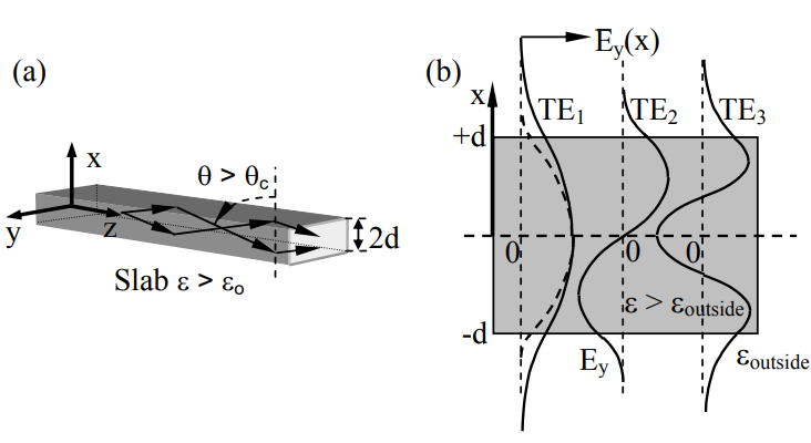
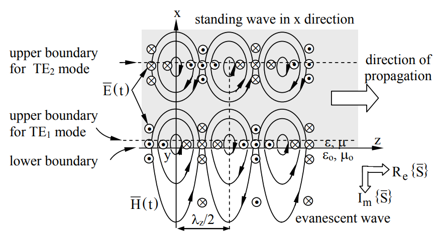
As discussed in Section 9.2.3, uniform plane waves within the dielectric are perfectly reflected at the slab boundary if they are incident beyond the critical angle \(\theta_{\mathrm{c}}=\sin ^{-1}\left(\mathrm{c}_{\varepsilon} / \mathrm{c}_{\mathrm{o}}\right) \), where c_ε and c_o are the velocities of light in the dielectric and outside, respectively. Such a wave and its perfect reflection propagate together along the z axis and form a standing wave in the orthogonal x direction. Outside the waveguide the waves are evanescent and decay exponentially away from the guide, as illustrated in Figure 12.2.2. This figure portrays the fields inside and outside the lower half of a dielectric slab having ε > ε_o; the lower boundary is at x = 0. The figure suggests two possible positions for the upper slab boundary that satisfy the boundary conditions for the TE₁ and TE₂ modes. Note that the TE₁ mode waveguide can be arbitrarily thin relative to λ and still satisfy the boundary conditions. The field configurations above the upper boundary mirror the fields below the lower boundary, but are not illustrated here. These waveguide modes are designated TE_n because the electric field is only transverse to the direction of propagation, and there is part of n half-wavelengths within the slab. The orthogonal modes (not illustrated) are designated TM_n.

Figure \(\PageIndex{2}\): Fields in dielectric slab waveguides for TE_n modes.

The fields inside a dielectric slab waveguide have the same form as (9.3.6) and (9.3.7) inside parallel-plate waveguides, although the boundary positions are different; also see Figures 9.3.1 and 9.3.3. If we define x = 0 at the axis of symmetry, and the thickness of the guide to be 2d, then within the guide the electric field for TE modes is:

\[\underline{\mathrm{\overline E}}=\hat{y} \underline{\mathrm{E}}_{\mathrm{o}}\left\{\sin \mathrm{k}_{\mathrm{x}} \mathrm{x} \textit { or } \operatorname{cosk}_{\mathrm{x}} \mathrm{x}\right\} \mathrm{e}^{-\mathrm{j} \mathrm{k}_{\mathrm{z}} \mathrm{z}} \qquad\qquad\qquad \text { for }|\mathrm{x}| \leq \mathrm{d} \label{12.2.1}\]

The fields outside are the same as for TE waves incident upon dielectric interfaces beyond the critical angle, (9.2.33) and (9.2.34):

\[\overline{\mathrm{\underline E}}=\hat{y} \underline{\mathrm{E}}_{1} \mathrm{e}^{-\alpha \mathrm{x}-\mathrm{j} \mathrm{k}_{\mathrm{z}} \mathrm{z}} \qquad\qquad\qquad \text { for } \mathrm{x} \geq \mathrm{d} \label{12.2.2}\]

\[\underline{\mathrm{\overline E}}=\{- \ \textit{or} \ +\} \hat{y} \mathrm{\underline E}_{1}^{+\alpha \mathrm{x}-\mathrm{jk}_{\mathrm{z}} \mathrm{z}} \qquad \qquad \qquad \mathrm{x} \leq \mathrm{-d} \label{12.2.3}\]

The first and second options in braces correspond to anti-symmetric and symmetric TE modes, respectively. Since the waves decay away from the slab, \(\alpha\) is positive. Faraday’s law in combination with (\ref{12.2.1}), (\ref{12.2.2}), and (\ref{12.2.3}) yields the corresponding magnetic field inside and outside the slab:

\[\begin{array}\overline{\mathrm{H}}=&\left[\hat{x} \mathrm{k}_{\mathrm{z}}\left\{\sin \mathrm{k}_{\mathrm{x}} \mathrm{x} \textit { or } \cos \mathrm{k}_{\mathrm{x}} \mathrm{x}\right\}\right.\\&\left.+\hat{z} \mathrm{jk}_{\mathrm{x}}\left\{\cos \mathrm{k}_{\mathrm{x}} \mathrm{x} \textit { or } \sin \mathrm{k}_{\mathrm{x}} \mathrm{x}\right\}\right]\left(\mathrm{\underline E}_{\mathrm{o}} / \omega \mu_{\mathrm{o}}\right) \mathrm{e}^{-\mathrm{j} \mathrm{k}_{\mathrm{z}} \mathrm{z}}\end{array} \qquad \qquad \qquad \text { for }|\mathrm{x}| \leq \mathrm{d} \label{12.2.4}\]

\[\overline{\mathrm{\underline H}}=-\left(\hat{x} \mathrm{k}_{\mathrm{z}}+\hat{z} \mathrm{j} \alpha\right)\left(\mathrm{\underline E}_{1} / \omega \mu_{\mathrm{o}}\right) \mathrm{e}^{-\alpha \mathrm{x}-\mathrm{j} \mathrm{k}_{\mathrm{z}} \mathrm{z}} \qquad\qquad\qquad \text { for } \mathrm{x} \geq \mathrm{d} \label{12.2.5}\]

\[\overline{\mathrm{\underline H}}=\{+\textit { or }-\}\left(\hat{x} \mathrm{k}_{\mathrm{z}}-\hat{z} \mathrm{j} \alpha\right)\left(\mathrm{\underline E}_{1} / \omega \mu_{\mathrm{o}}\right) \mathrm{e}^{\alpha \mathrm{x}-\mathrm{j} \mathrm{k}_{\mathrm{z}} \mathrm{z}} \qquad \qquad \qquad \text { for } \mathrm{x} \leq-\mathrm{d} \label{12.2.6}\]

The TE₁ mode has the interesting property that it approaches TEM behavior as ω → 0 and the decay length approaches infinity; most of the energy is then propagating outside the slab even though the mode is guided by it. Modes with n ≥ 2 have non-zero cut-off frequencies. There is no TM mode that propagates for f→0 in dielectric slab waveguides, however.

Although Figure 12.2.1(a) portrays a slab with an insulating medium outside, the first option in brackets {•} for the field solutions above is also consistent for x > 0 with a slab located 0 < x < d and having a perfectly conducting wall at x = 0; all boundary conditions are matched; these are the anti-symmetric TE modes. This configuration corresponds, for example, to certain optical guiding structures overlaid on conductive semiconductors.

To complete the TE field solutions above we need additional relations between \( \underline{\mathrm{E}}_{\mathrm o}\) and \(\underline{\mathrm{E}}_{1} \), and between k_x and \(\alpha\). Matching \( \overline{\mathrm{\underline E}}\) at x = d for the symmetric solution [cos k_xx in (\ref{12.2.1})] yields:

\[\mathrm{\hat{y} \underline{E}_{0} \cos \left(k_{x} d\right) e^{-j k_{z} z}=\hat{y} \underline{E}_{1} e^{-\alpha d-j k_{z} z}} \label{12.2.7}\]

Matching the parallel (\(\hat{\mathrm z}\)) component of \(\overline{\mathrm{\underline H}}\) at x = d yields:

\[-\hat{\mathrm z} j \mathrm{k}_{\mathrm{x}} \sin \left(\mathrm{k}_{\mathrm{x}} \mathrm{d}\right)\left(\underline{\mathrm{E}}_{\mathrm{o}} / \omega \mu_{\mathrm{o}}\right) \mathrm{e}^{-\mathrm{j} \mathrm{k}_{\mathrm{z}} \mathrm{z}}=-\hat{\mathrm z} \mathrm{j} \alpha\left(\mathrm{\underline E}_{1} / \omega \mu_{\mathrm{o}}\right) \mathrm{e}^{-\alpha \mathrm{d}-\mathrm{j} \mathrm{k}_{\mathrm{z}} \mathrm{z}} \label{12.2.8}\]

The guidance condition for the symmetric TE dielectric slab waveguide modes is given by the ratio of (\ref{12.2.8}) to (\ref{12.2.7}):

\[\mathrm{k}_{\mathrm{x}} \mathrm{d} \tan \left(\mathrm{k}_{\mathrm{x}} \mathrm{d}\right)=\alpha \mathrm{d} \qquad \qquad \qquad \text{(slab guidance condition) } \label{12.2.9}\]

Combining the following two dispersion relations and eliminating k_z can provide the needed additional relation (\ref{12.2.12}) between k_x and \(\alpha\):

\[\mathrm{k}_{\mathrm{Z}}^{2}+\mathrm{k}_{\mathrm{x}}^{2}=\omega^{2} \mu_{\mathrm{o}} \varepsilon \qquad \qquad \qquad \text{(dispersion relation inside)} \label{12.2.10}\]

\[\mathrm{k}_{\mathrm{Z}}^{2}-\alpha^{2}=\omega^{2} \mu_{\mathrm{o}} \varepsilon_{\mathrm{o}} \qquad \qquad \qquad \text{(dispersion relation outside) } \label{12.2.11}\]

\[\mathrm{k}_{\mathrm{x}}^{2}+\alpha^{2}=\omega^{2}\left(\mu_{\mathrm{o}} \varepsilon-\mu_{\mathrm{o}} \varepsilon_{\mathrm{o}}\right)>0 \qquad \qquad \qquad \text{(slab dispersion relation) } \label{12.2.12}\]

By substituting into the guidance condition (\ref{12.2.9}) the expression for \(\alpha\) that follows from the slab dispersion relation (\ref{12.2.12}) we obtain a transcendental guidance equation that can be solved numerically or graphically:

\[\tan \mathrm{k}_{\mathrm{x}} \mathrm{d}=\left(\left[\omega^{2} \mu_{\mathrm{o}}\left(\varepsilon-\varepsilon_{\mathrm{o}}\right) \mathrm{d}^{2} / \mathrm{k}_{\mathrm{x}}^{2} \mathrm{d}^{2}\right]-1\right)^{0.5} \qquad\qquad\qquad \text { (guidance equation) } \label{12.2.13}\]

Figure 12.2.3 plots the left- and right-hand sides of (\ref{12.2.13}) separately, so the modal solutions are those values of k_xd for which the two families of curves intersect.

Figure \(\PageIndex{3}\): TE modes for a dielectric slab waveguide.

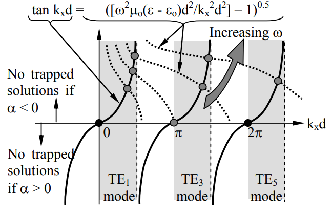
Note that the TE₁ mode can be trapped and propagate at all frequencies, from nearly zero to infinity. At low frequencies the waves guided by the slab have small values of \(\alpha\) and decay very slowly away from the slab so that most of the energy is actually propagating in the z direction outside the slab rather than inside. The value of \(\alpha\) can be found from (\ref{12.2.12}), and it approaches zero as both k_xd and ω approach zero.

The TE₃ mode cannot propagate near zero frequency however. Its cutoff frequency \(\omega_{\mathrm{TE} 3}\) occurs when k_xd = \(\pi\), as suggested by Figure 12.2.3; \( \omega_{\mathrm{TE} 3}\) can be determined by solving (\ref{12.2.12}) for this case. This and all higher modes cannot be trapped at low frequencies because then the plane waves that comprise them impact the slab wall at angles beyond \( \theta_{\mathrm{c}}\) that permit escape. As ω increases, more modes can propagate. Figures 12.2.2 and 12.2.1(b) illustrate symmetric TE₁ and TE₃ modes, and the antisymmetric TE₂ mode. Similar figures could be constructed for TM modes.

These solutions for dielectric-slab waveguides are similar to the solutions for optical fibers, which instead take the form of Bessel functions because of their cylindrical geometry. In both cases we have lateral standing waves propagating inside and evanescent waves propagating outside.

Optical fibers

An optical fiber is generally a very long solid glass wire that traps lightwaves inside as do the dielectric slab waveguides described in Section 12.2.1. Fiber lengths can be tens of kilometers or more. Because the fiber geometry is cylindrical, the electric and magnetic fields inside and outside the fiber are characterized by Bessel functions, which we do not address here. These propagating electromagnetic fields exhibit lateral standing waves inside the fiber and evanescence outside. To minimize loss the fiber core is usually overlaid with a low-permittivity glass cladding so that the evanescent decay also occurs within low-loss glass.

A typical glass optical fiber transmission line is perhaps 125 microns in diameter with a high-permittivity glass core having diameter ~6 microns. The core permittivity ε + Δε is typically ~2 percent greater than that of the cladding (ε). If the lightwaves within the core impact the cladding beyond the critical angle θ_c, where:

\[\theta_{\mathrm{c}}=\sin ^{-1}(\varepsilon /(\varepsilon+\Delta \varepsilon)) \label{12.2.14}\]

then these waves are perfectly reflected and trapped. The evanescent waves inside the cladding decay approximately exponentially away from the core to negligible values at the outer cladding boundary, which is often encased in plastic about 0.1 mm thick that may be reinforced. Gradedindex fibers have a graded transition in permittivity between the core and cladding. Some fibers propagate multiple modes that travel at different velocities so as to interfere at the output and limit information extraction (data rate). Multiple fibers are usually bundled inside a single cable. Figure 12.2.4 suggests the structure of a typical fiber.

Figure \(\PageIndex{4}\): Typical clad optical fiber.

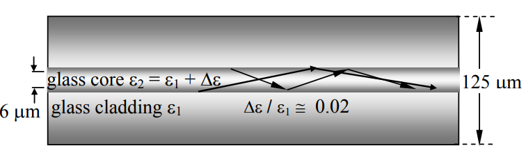
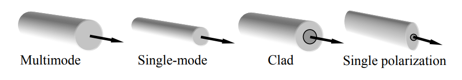
Figure 12.2.5 shows four common forms of optical fiber; many others exist. The multimode fiber is thicker and propagates several modes, while the single-mode fiber is so thin that only one mode can propagate. The diameter of the core determines the number of propagating modes. In all cylindrical structures, even single-mode fibers, both vertically and horizontally polarized waves can propagate independently and therefore may interfere with each other when detected at the output. If a single-mode fiber has an elliptical cross-section, one polarization can be made to escape so the signal becomes pure. That is, one polarization decays more slowly away from the core so that it sees more of the absorbing material that surrounds the cladding.

Figure \(\PageIndex{5}\): Types of optical fiber.

The initial issue faced in the 1970’s by designers of optical fibers was propagation loss. Most serious was absorption due to residual levels of impurities in the glass, so much research and development involved purification. Water posed a particularly difficult problem because one of its harmonics fell in the region where attenuation in glass was otherwise minimum, as suggested in Figure 12.2.6.

Figure \(\PageIndex{6}\): Loss mechanisms in optical fibers.

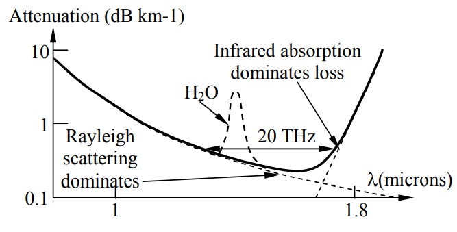
At wavelengths shorter than ~1.5 microns the losses are dominated by Rayleigh scattering of the waves from the random fluctuations in glass density on atomic scales. These scattered waves exit the fiber at angles less than the critical angle. Rayleigh scattering is proportional to f⁴ and occurs when the inhomogeneities in ε are small compared to λ/2\(\pi\). Inhomogeneities in glass fibers have near-atomic scales, say 1 nm, whereas the wavelength is more than 1000 times larger. Rayleigh scattering losses are reduced by minimizing unnecessary inhomogeneities through glass purification and careful mixing, and by decreasing the critical angle. Losses due to scattering by rough fiber walls are small because drawn glass fibers can be very smooth and little energy impacts the walls.

At wavelengths longer than ~1.5 microns the wings of infrared absorption lines at lower frequencies begin to dominate. This absorption is due principally to the vibration spectra of inter-atomic bonds, and is unavoidable. The resulting low-attenuation band centered near 1.5­ microns between the Rayleigh and IR attenuating regions is about 20 THz wide, sufficient for a single fiber to provide each person in the U.S.A. with a bandwidth of 20×10¹²/2.5×10⁸ = 80 kHz, or 15 private telephone channels! Most fibers used for local distribution do not operate anywhere close to this limit for lack of demand, although some undersea cables are pushing toward it.

The fibers are usually manufactured first as a preform, which is a glass rod that subsequently can be heated at one end and drawn into a fiber of the desired thickness. Preforms are either solid or hollow. The solid ones are usually made by vapor deposition of SiO₂ and GeO₂ on the outer surface of the initial core rod, which might be a millimeter thick. By varying the mixture of gases, usually Si(Ge)Cl₄ + O₂ ⇒ Si(Ge)O₂ + 2Cl₂, the permittivity of the deposited glass cladding can be reduced about 2 percent below that of the core. The boundary between core and cladding can be sharp or graded in a controlled way. Alternatively, the preform cladding is large and hollow, and the core is deposited from the inside by hot gases in the same way; upon completion there is still a hole through the middle of the fiber. Since the core is small compared to the cladding, the preforms can be made more rapidly this way. When the preform is drawn into a fiber, any hollow core vanishes. Sometimes a hollow core is an advantage. For example, some newer types of fibers have cores with laterally-periodic lossless longitudinal hollows within which much of the energy can propagate.

Another major design issue involves the fiber dispersion associated with frequency dependent phase and group velocities, where the phase velocity v_p = ω/k. If the group velocity v_g, which is the velocity of the envelope of a narrow band sinusoid, varies over the optical bandwidth, then the signal waveform will increasingly distort as it propagates because the faster moving frequency components of the envelope will arrive early. For example, a digital pulse of light that lasts T seconds is produced by multiplying a boxcar modulation envelope (the T second pulse shape) by the sinusoidal optical carrier, so the frequency spectrum is the convolution of the spectrum for the sinusoid (a spectral impulse) and the spectrum for a boxcar pulse (∝ [sin(2\(\pi\)t/T)]/[2\(\pi\)t/T]). The outermost frequencies suffer from dispersion the most, and these are primarily associated with the sharp edges of the pulse.

The group velocity v_g derived in (9.5.20) is the slope of the dispersion relation at the optical frequency of interest:

\[\mathrm{v}_{\mathrm{g}}=(\partial \mathrm{k} / \partial \omega)^{-1} \label{12.2.15}\]

Figure 12.2.7 illustrates the dispersion relation for three different modes; the higher order modes propagate information more slowly.

Figure \(\PageIndex{7}\): Group velocities for optical fiber modes.

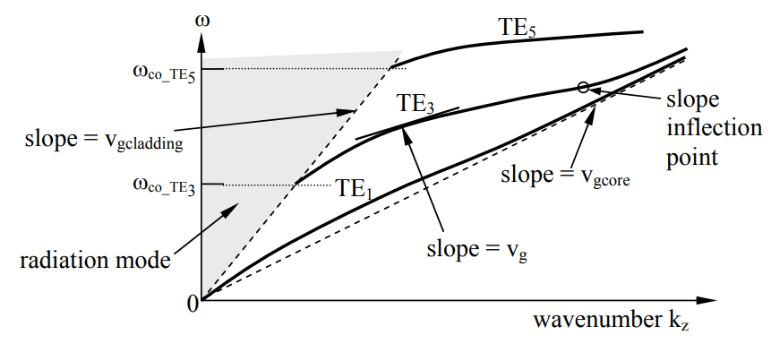
The group velocity v_g is the slope of the ω(k) relation and is bounded by the slopes associated with the core (v_gcore) and with the cladding (v_gcladding), where the cladding is assumed to be infinite. The figure has greatly exaggerated the difference in the slope between the core and cladding for illustrative purposes.

A dispersive line eventually transforms a square optical pulse into a long “frequency chirped” pulse with the faster propagating frequencies in the front and the slower propagating frequencies in the back. This problem can be minimized by carefully choosing combinations of: 1) the dispersion n(f) of the glass, 2) the permittivity contour ε(r) in the fiber, and 3) the optical center frequency f_o. Otherwise we must reduce either the bandwidth of the signal or the length of the fiber. To increase the distance between amplifiers the dispersion can be compensated periodically by special fibers or other elements with opposite dispersion.

Pulses spread as they propagate over distance L because their outermost frequency components ω₁ and ω₂ = ω₁+Δω have arrival times at the output separated by:

\[\Delta \mathrm{t}=\mathrm{L} / \mathrm{v}_{\mathrm{gl}}-\mathrm{L} / \mathrm{v}_{\mathrm{g} 2}=\mathrm{L}\left[\mathrm{d}\left(\mathrm{v}_{\mathrm{g}}^{-1}\right) / \mathrm{d} \omega\right] \Delta \omega=\mathrm{L}\left(\mathrm{d}^{2} \mathrm{k} / \mathrm{d} \omega^{2}\right) \Delta \omega \label{12.2.16}\]

where v_gi is the group velocity at ω_i (\ref{12.2.15}). Typical pulses of duration T_p have a bandwidth \(\Delta \omega \cong \mathrm{T_{p}^{-1}}\), so brief pulses spread faster. The spread Δt is least at frequencies where d²k/dω² ≅ 0, which is near the representative slope inflection point illustrated in Figure 12.2.7.

This natural fiber dispersion can, however, help solve the problem of fiber nonlinearity. Since attenuation is always present in the fibers, the amplifiers operate at high powers, limited partly by their own nonlinearities and those in the fiber that arise because ε depends very slightly on the field strength E. The effects of non-linearities are more severe when the signals are in the form of isolated high-energy pulses. Deliberately dispersing and spreading the isolated pulses before amplifying and introducing them to the fiber reduces their peak amplitudes and the resulting nonlinear effects. This pre-dispersion is made opposite to that of the fiber so that the fiber dispersion gradually compensates for the pre-dispersion over the full length of the fiber. That is, if the fiber propagates high frequencies faster, then those high frequency components are delayed correspondingly before being introduced to the fiber. When the pulses reappear in their original sharp form at the far end of the fiber their peak amplitudes are so weak from natural attenuation that they no longer drive the fiber nonlinear.

Example \(\PageIndex{A}\)

If 10-ps pulses are used to transmit data at 20 Gbps, they would be spaced 5×10^-10 sec apart and would therefore begin to interfere with each other after propagating a distance L_max sufficient to spread those pulses to widths of 50 ps. A standard single-mode optical fiber has dispersion d²k/dω² of 20 ps²/km at 1.5 μm wavelength. At what distance L_max will such 10-ps pulses have broadened to 50 ps?

Solution

Using (12.2.16) and \( \Delta \omega \cong \mathrm{T_{p}^{-1}}\) we find:

\[\mathrm{L}_{\mathrm{max}}=\Delta \mathrm{t} /\left[\Delta \omega\left(\mathrm{d}^{2} \mathrm{k} / \mathrm{d} \omega^{2}\right)\right]=50 \ \mathrm{ps} \times 10\ \mathrm{ps} /\left(20 \ \mathrm{ps}^{2} / \mathrm{km}\right)=25 \ \mathrm{km} \nonumber\]

Thus we must slow this fiber to 10 Gbps if the amplifiers are 50 km apart.