8.3: Distortions due to loss and dispersion

Lossy transmission lines

In most electronic systems transmission line loss is a concern because business strategy generally dictates reducing wire diameters and costs until such issues arise. For example, the polysilicon often used for conductors in integrated silicon devices has noticeable resistance.

The TEM circuit model of Figure 8.3.1 incorporates two types of loss. The series resistance R per meter arises from the finite conductivity of the wires, while the parallel conductance G per meter arises from leakage currents flowing between the wires through the medium separating them.

Figure \(\PageIndex{1}\): Distributed circuit model for lossy TEM transmission lines.

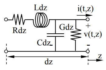
When these lossy elements are included, we obtain the telegraphers’ equations:

\[\mathrm{dv} / \mathrm{dz}=-\mathrm{Ri}-\mathrm{L} \mathrm{di} / \mathrm{dt} \qquad \qquad \qquad \text{(telegraphers’ equation)} \nonumber \]

\[\mathrm{di} / \mathrm{dz}=-\mathrm{Gv}-\mathrm{Cdv} / \mathrm{dt} \qquad \qquad \qquad \text{(telegraphers’ equation)} \nonumber \]

If the wires are resistive, then current flowing through them introduces longitudinal electric fields E_z, violating the TEM assumption: E_z = H_z = 0. Since rigorous solution of Maxwell’s equations for the non-TEM case is challenging, the telegraphers’ equations are often used instead if the loss is modest. The same problem does not arise with G because it does not violate the TEM assumption, as shown in Section 7.1.3. Since propagation in such lossy TEM lines is frequency dependent, the telegraphers’ equations (8.3.1–2) and their solutions are generally expressed using complex notation⁴⁵:

\[\mathrm{d} \underline{\mathrm{V}}(\mathrm{z}) / \mathrm{dz}=-(\mathrm{R}+\mathrm{j} \omega \mathrm{L}) \mathrm{\underline I}(\mathrm{z}) \qquad \qquad \qquad \text{(telegraphers’ equation)} \nonumber \]

\[\mathrm{d} \underline{\mathrm{I}}(\mathrm{z}) / \mathrm{dz}=-(\mathrm{G}+\mathrm{j} \omega \mathrm{C}) \mathrm{\underline V}(\mathrm{z}) \qquad \qquad \qquad \text{(telegraphers’ equation) } \nonumber \]

⁴⁵ Complex notation is discussed in Section 2.3.2 and Appendix B. In general, \(\mathrm{v}(\mathrm{t})=\mathrm{R}_{\mathrm{e}}\left\{\underline{\mathrm{V}} \mathrm{e}^{\mathrm{j} \omega \mathrm{t}}\right\}\), where \(R_{e}\left\{\bullet e^{j \omega t}\right\}\) is omitted from equations.

Differentiating (8.3.3) with respect to z, and substituting (8.3.4) for \(\mathrm{d} \underline{\mathrm{I}}(\mathrm{z}) / \mathrm{dz}\) yields the wave equation for lossy TEM lines, where the sign of k² is chosen so that k is real, consistent with the lossless solutions discussed earlier in Section 7.1.2:

\[\mathrm{d}^{2} \mathrm{\underline V}(\mathrm{z}) / \mathrm{dz}^{2}=(\mathrm{R}+\mathrm{j} \omega \mathrm{L})(\mathrm{G}+\mathrm{j} \omega \mathrm{C}) \mathrm{\underline V}(\mathrm{z})=-\mathrm{k}^{2} \mathrm{\underline V}(\mathrm{z}) \qquad \qquad \qquad \text { (wave equation) } \nonumber \]

\[\mathrm{\underline{k}=[-(R+j \omega L)(G+j \omega C)]^{0.5}=k^{\prime}-j k^{\prime \prime}} \qquad\qquad\qquad \text { (TEM propagation constant) } \nonumber \]

Since the second derivative of \(\mathrm{\underline{V}(z)}\) equals a constant times itself, it must be expressible as the sum of exponentials that have this property:

\[\mathrm{\underline{V}(z)=\underline{V}_{+} \mathrm{e}^{-j \underline{\mathrm{k}} z}+\underline{\mathrm{V}}_{-} \mathrm{e}^{+j \mathrm{\underline k}z}} \qquad \qquad \qquad \text { (TEM voltage solution) } \nonumber \]

Differentiating (8.3.7) with respect to z and substituting the result in (8.3.3) yields both \(\mathrm{\underline{I}(z)}\) and \(\mathrm{\underline{Y}_{0}}\):

\[\mathrm{\underline{I}(z)=\underline{Y}_{0}\left(\underline{V}_{+} \mathrm{e}^{-\mathrm{j} \mathrm{\underline k} \mathrm{z}}-\underline{\mathrm{V}}_{-} \mathrm{e}^{+j \mathrm{\underline k} z}\right)} \qquad\qquad\qquad(\text {TEM current solution}) \nonumber \]

\[\mathrm{\underline{Z}_{0}=\frac{1}{\underline{Y}_{0}}=\sqrt{\frac{R+j \omega L}{G+j \omega C}}} \qquad\qquad\qquad(\text {characteristic impedance}) \nonumber \]

When R = G = 0, (8.3.9) reduces to the well known result Z_o = (L/C)^0.5.

Thus two new properties emerge when TEM lines are dissipative: 1) because \(\mathrm{\underline{k}}\) is complex and a non-linear function of frequency, waves are attenuated and dispersed as they propagate in a frequency-dependent manner, and 2) \(\underline{\mathrm{Z}}_{0}\) is complex and frequency dependent. Both k' and k" (8.3.6) are functions of frequency, so signals propagating on lossy lines change shape, partly because different frequency components propagate and decay differently. The resulting attenuation and dispersion are discussed in Sections 8.3.1 and 8.3.2, respectively. Reflections are affected at junctions by losses, and also are attenuated with distance so the impedance of a lossy line \(\underline{\mathrm{Z}}(\mathrm{z}) \rightarrow \underline{\mathrm{Z}}_{0}\) regardless of load as \(\mathrm{\underline{V}_{-}(z)}\) becomes negligible. Reflections by junctions involving lossy lines are simply analyzed by replacing Z_o by a complex impedance \( \underline{\mathrm{Z}}_{0}\) in the expressions developed in Section 7.2 for lossless lines.

Waves propagating only in the +z direction obey (8.3.7), which becomes:

\[\mathrm{\underline{V}(z)=\underline{V}_{+} \mathrm{e}^{-j \underline{k} z}=\underline{V}_{+} \mathrm{e}^{-j \mathrm{k}^{\prime} z} \mathrm{e}^{-\mathrm{k}^{\prime \prime} z}} \qquad\qquad\qquad \text { (decaying propagating wave) } \nonumber \]

One combination of R, L, C, and G is particularly interesting because it results in zero dispersion and a frequency-independent decay that does not distort waveforms. We may discover this combination by evaluating \(\underline{\mathrm{k}}\) using (8.3.6):

\[\mathrm{\underline{k}=[-(R+j \omega L)(G+j \omega C)]^{0.5}=\omega\{L C[1-j(R / \omega L)][1-j(G / \omega C)]\}^{0.5}} \nonumber \]

It follows from (8.3.11) that if R/L = G/C, then the phase velocity (v_p = ω/k' = [LC]^-0.5) and the decay rate (k" = R[C/L]^0.5) are both frequency independent:

\[\mathrm{\underline k}=(\mathrm{LC})^{0.5}(\omega-\mathrm{jR} / \mathrm{L})=\mathrm{k}^{\prime}-\mathrm{jk}^{\prime \prime} \qquad \qquad \qquad \text{(distortionless line)} \nonumber \]

The ability to avoid signal distortion due to frequency-dependent absorption was first exploited by telephone companies who added small inductors periodically in series with their longer phone lines in order to reduce R/L so that it balanced G/C; the result was called a distortionless line, and the coils are called Pupin coils after their inventor⁴⁶. The consequences of dispersion are explored in Section 8.3.2.

⁴⁶ Pupin coils had to be inserted at least every λ/10 meters in order to avoid additional distortions, but the shortest λ for telephone voice signals is ~c/f = 3×10⁸ /3000 = 100 km.

Another limit is sometimes of interest when the effects of R dominate those of ωL. This occurs, for example, in resistive polysilicon or diffusion lines in integrated circuits, which may be approximately modeled by eliminating L and G from Figure 8.3.1. Then \(\underline{\mathrm{k}}\) (8.3.11) becomes:

\[\mathrm{\underline{k} \cong(-j \omega R C)^{0.5}=(\omega R C / 2)^{0.5}-j(\omega R C / 2)^{0.5}=k^{\prime}-j k^{\prime \prime}} \nonumber \]

The square root of -j was chosen to correspond to a decaying wave rather than to exponential growth. The phase and group velocities for this line are the same:

\[\mathrm{v}_{\mathrm{p}}=\omega / \mathrm{k}^{\prime}=(2 \omega / \mathrm{RC})^{0.5} \ \left[\mathrm{m} \mathrm{s}^{-1}\right] \nonumber \]

\[\mathrm{v}_{\mathrm{g}}=\left(\partial \mathrm{k}^{\prime} / \partial \omega\right)^{-1}=2(\omega / \mathrm{RC})^{0.5} \ \left[\mathrm{m} \mathrm{s}^{-1}\right] \nonumber \]

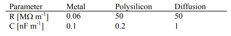
Although it is not easy to relate these frequency-dependent velocities to delays in digital circuits, they demonstrate that such delays exist and express their dependence on R and C. That is, larger line time constants RC lower pulse velocities and increase delays. Such lines are best used when they are short compared to the shortest wavelength of interest, D < λ = v_p/f_max = 2\(\pi\)(2/rcω_max)^0.5. In polysilicon lines λ_min ≅ 1 mm for ω_max = 10¹⁰. The response to arbitrary waveform excitation can be computed by: 1) Fourier transforming the signal, 2) propagating each frequency component as dictated by (8.3.13), and then 3) reconstructing the signal at the new location with an inverse Fourier transform. Typical values for R and C in metal, polysilicon, and diffusion lines are presented in Table 8.3.1, and correspond to velocities much less than c. The costs of these three options for forming conductors are unequal and must also be considered when designing fast integrated circuits.

Table \(\PageIndex{1}\): Resistance and capacitance per meter for typical integrated circuit lines.

Provided R is not so large compared to ωL that the TEM approximation is invalid because of strong longitudinal electric fields, then the power dissipated is:

\[\mathrm{P}_{\mathrm{d}}=\left(\left.\mathrm{R}\left|\underline{\mathrm{I}}^{2}+\mathrm{G}\right| \mathrm{\underline V}\right|^{2}\right) / 2 \ \left[\mathrm{W} \mathrm{m}^{-1}\right] \nonumber \]

Dispersive transmission lines

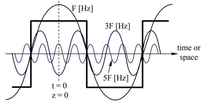
Different frequency components propagate at different velocities on dispersive transmission lines. The nature and consequences of dispersion are discussed further in Section 9.5.2. Consider first a square-wave computer clock pulse at F Hz propagating along a dispersive TEM line. The Fourier transform of this signal has its fundamental at F Hz, with odd harmonics at 3F, 5F, etc., each of which has its own phase velocity, as suggested in Figure 8.3.2.

Figure \(\PageIndex{2}\): Square wave and its constituent sinusoids.

Significant pulse distortion occurs if a strong harmonic is shifted as much as ~90^o relative to the fundamental. To determine the relative phase shift between fundamental and harmonic we can first multiply the difference in phase velocity at F and 3F, e.g., v_pF - v_p3F, by the propagation time T of interest. This yields the spatial offset between these two harmonics, which we might limit to λ/4 for 3F. That is, we might expect significant distortion over a transmission line of length D = v_pT meters if:

\[\left(\mathrm{v}_{\mathrm{pF}}-\mathrm{v}_{\mathrm{p} 3 \mathrm{F}}\right) \mathrm{T}>\sim \lambda_{3 \mathrm{F}} / 4=\mathrm{v}_{\mathrm{p} 3 \mathrm{F}} /(4 \times 3 \mathrm{F}) \nonumber \]

There is a similar limit to the propagation distance of narrowband pulse signals before waveform distortion becomes unacceptable. Digital communications systems commonly use narrowband pulses s(t) for both wireless and cable signaling. For example, the square wave in Figure 8.3.2 could also represent the amplitude envelope \(\mathrm{A}(\mathrm{t})=\Sigma_{\mathrm{i}} \mathrm{a}_{\mathrm{i}} \cos \omega_{\mathrm{i}} \mathrm{t}\) of an underlying sinusoid cosω_ot, where ω_o >> ω_i>0 and together they occupy a narrow bandwidth. That is:

\[\mathrm{s}(\mathrm{t})=\left(\cos \omega_{\mathrm{o}} \mathrm{t}\right) \sum_{\mathrm{i}=1} \mathrm{a}_{\mathrm{i}} \cos \omega_{\mathrm{i}} \mathrm{t}=0.5 \sum_{\mathrm{i}} \mathrm{a}_{\mathrm{i}}\left\{\cos \left[\left(\omega_{\mathrm{o}}+\omega_{\mathrm{i}}\right) \mathrm{t}+\cos \left[\left(\omega_{\mathrm{o}}-\omega_{\mathrm{i}}\right) \mathrm{t}\right]\right]\right\} \nonumber \]

Since each frequency ω_o±ω_i propagates at a slightly different phase velocity, a narrowband pulse will also distort when a strong harmonic is ~λ/4 out of phase relative to the original wave envelope, which is much larger than λ = 2\(\pi\)c/ω_o for narrowband signals. Some applications are more sensitive to dispersive distortion than others; for example, distorted digital signals can be generally be regenerated distortion free, while analog signals require inverse distortion, which is often uneconomic.

Distortion of narrowband signals is usually computed in terms of the group velocity v_g, which is the velocity of propagation for the waveform envelope and equals the velocity of energy or information, which can never exceed c, the velocity of light in vacuum. The sine wave that characterizes the average frequency of a narrowband pulse propagates at the phase velocity v_p, which can be greater or less than c. Narrowband pulse signals (e.g., digitally modulated sinusoids) distort when the accumulated difference Δ in the envelope propagation distances between the high- and low-frequency end of the signal spectrum differs by more than a small fraction of the minimum pulse width W[m] (e.g., the length of a zero or one). Since the difference in group velocity across the bandwidth B[Hz] is (∂v_g/∂f)B [m/s], and the pulse travel time is D/v_g, where D is propagation distance, it follows that the difference in envelope propagation distance across the band is:

\[\Delta=\frac{\partial \mathrm{v}_{\mathrm{g}}}{\partial \mathrm{f}} \frac{\mathrm{BD}}{\mathrm{V}_{\mathrm{g}}} \ [\mathrm{m}] \nonumber \]

Since the minimum pulse width W is ~v_g/B [m], the requirement that D << W implies that the maximum distortion-free propagation distance D is:

\[\mathrm{D} \ll\left(\frac{\mathrm{v}_{\mathrm{g}}}{\mathrm{B}}\right)^{2}\left(\frac{\partial \mathrm{v}_{\mathrm{g}}}{\partial \mathrm{f}}\right)^{-1} \nonumber \]

Group and phase velocity are discussed further in Section 9.5.2 and their effect on distortion is explored in Section 12.2.2.

Example \(\PageIndex{A}\)

Typical 50-ohm coaxial cables for home distribution of television and internet signals have series resistance R ≅ 0.02(f_MHz^0.5) ohms m^-1. Assume ε = 4ε_o, μ = μ_o. How far can signals propagate before attenuating 60 dB?

Solution

Since conductivity G ≅ 0, (8.3.11) says \(\mathrm{\underline{k}=\omega[L C(1-j R / \omega L)]^{0.5}=k^{\prime}+j k^{\prime \prime}}\). The imaginary part of \(\underline{\mathrm{k}}\) corresponds to exponential decay. For R << ωL, \(\mathrm{\underline{k} \cong \omega(L C)}^{0.5}(1-\mathrm{jR} / \omega \mathrm{L})^{0.5}\), so k" = -(ωRC)^0.5. To find C we note the phase velocity \(\mathrm{v}=\left(\mu_{\mathrm{o}} 4 \varepsilon_{\mathrm{o}}\right)^{-0.5}=(\mathrm{LC})^{-0.5}=\mathrm{c} / 2 \cong 1.5 \times 10^{8} \ \left[\mathrm{m} \mathrm{s}^{-1}\right]\), and Z_o = 50 = (L/C)^0.5. Therefore \(\mathrm{C=2 / c Z_{0}}=2 /\left(3 \times 10^{8} \times 50\right) \cong 1.33 \times 10^{-10} \ [\mathrm F]\). Thus at 100 MHz, \(\mathrm{k}^{\prime \prime}=-(\omega \mathrm{RC})^{0.5}=-\left(2 \pi 10^{8} \times 0.2 \times 1.33 \times 10^{-10}\right)^{0.5} \cong-0.017\). Since power decays as e^-2k"z , 60 dB corresponds to e^-2k"z = 10^-6, so z = -ln(10^-6)/2k" = 406 meters. At 100 MHz the approximation R << ωL is quite valid. As coaxial cable systems boost data rates and their maximum frequency above 100-200 MHz, the increased attenuation requires amplifiers at intervals so short as to motivate switching to optical fibers that can propagate signals hundred of kilometers without amplification.