13.2: Acoustic waves at interfaces and in guiding structures and resonators

Boundary conditions and waves at interfaces

The behavior of acoustic waves at boundaries is determined by the acoustic boundary conditions. At rigid walls the normal component of acoustic velocity must clearly be zero, and fluid pressure is unconstrained there. At boundaries between two fluids or gases in equilibrium, both the acoustic pressure \( \mathrm{p}(\overline{\mathrm{r}}, \mathrm{t})\) and the normal component of acoustic velocity \(\overline{\mathrm{u}}_{\perp}(\overline{\mathrm{r}}, \mathrm{t}) \) must be continuous. If the pressure were discontinuous, then a finite force normal to the interface would be acting on infinitesimal mass, giving it infinite acceleration, which is not possible. If were discontinuous, then ∂p/∂t at the interface would be infinite, which also is not possible; (13.1.8) says \( \nabla \bullet \overline{\mathrm{u}}=-\left(1 / \gamma \mathrm{P}_{\mathrm{o}}\right) \partial \mathrm{p} / \partial \mathrm{t}\). These acoustic boundary conditions at a boundary between media 1 and 2 can be stated as:

\[\mathrm{p_{1}=p_{2}} \qquad \qquad \qquad \text { (boundary condition for pressure) } \label{13.2.1}\]

\[\overline{\mathrm{u}}_{1 \perp}=\overline{\mathrm{u}}_{2 \perp} \qquad \qquad \qquad \text { (boundary condition for velocity) } \label{13.2.2}\]

A uniform acoustic plane wave incident upon a planar boundary between two media having different acoustic properties will generally have a transmitted component and a reflected component, as suggested in Figure 13.2.1. The angles of incidence, reflection, and transmission are θ_i, θ_r, and θ_t, respectively.

Figure \(\PageIndex{1}\): Acoustic waves at a planar interface with phase matching.

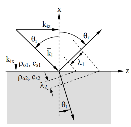
A typical example is the boundary between cold air overlying a lake and warm air above; the warm air is less dense, although the pressures across the boundary must balance. Since \(\mathrm{c}_{\mathrm{s}} \propto \rho_{\mathrm{o}}^{-0.5}\) and \(\eta_{\mathrm{s}} \propto \rho_{\mathrm{o}}^{ \ 0.5}\), both the amplitudes and angles of propagation must change at the density discontinuity.

As was done for electromagnetic waves (see Section 9.2.2), we can begin with tentative general expressions for the incident, reflected, and transmitted plane waves:

\[\underline{\mathrm{p}}_{\mathrm{i}}(\overline{\mathrm{r}})=\underline{\mathrm{p}}_{\mathrm{io}} \mathrm{e}^{+\mathrm{j} \mathrm{k}_{\mathrm{ix}} \mathrm{x}-\mathrm{j} \mathrm{k}_{\mathrm{iz}^{\mathrm z}}} \qquad \qquad \qquad \text{(incident wave) } \label{13.2.3}\]

\[\underline{\mathrm{p}}_{\mathrm{r}}(\overline{\mathrm{r}})=\underline{\mathrm{p}}_{\mathrm{ro}} \mathrm{e}^{+\mathrm{j} \mathrm{k}_{\mathrm{rx}} \mathrm{x}-\mathrm{j} \mathrm{k}_{\mathrm{rz}}^{\ \mathrm z}} \qquad \qquad \qquad \text{(reflected wave) } \label{13.2.4}\]

\[\underline{\mathrm{p}}_{\mathrm{t}}(\overline{\mathrm{r}})=\underline{\mathrm{p}}_{\mathrm{to}} \mathrm{e}^{+\mathrm{j} \mathrm{k}_{\mathrm{tx}} \mathrm{x}-\mathrm{jk}_{\mathrm{t} \mathrm{z}}^{\ \mathrm{z}}} \label{13.2.5}\]

At x = 0 the pressure is continuous across the boundary (\ref{13.2.1}), so \(\mathrm{\underline{p}_{i}(\bar{r})+\underline{p}_{r}(\bar{r})=\underline{p}_{t}(\bar{r})} \), which requires the phases (-jkz) to match:

\[\mathrm{k}_{\mathrm{iz}}=\mathrm{k}_{\mathrm{rz}}=\mathrm{k}_{\mathrm{tz}} \equiv \mathrm{k}_{\mathrm{z}} \label{13.2.6}\]

But k_z is the projection of the \(\overline{\mathrm{k}} \) on the z axis, so k_iz = k_isin θ_i, where k_i = ω/c_si, and:

\[\mathrm{k}_{\mathrm{i}} \sin \theta_{\mathrm{i}}=\mathrm{k}_{\mathrm{r}} \sin \theta_{\mathrm{r}}=\mathrm{k}_{\mathrm{t}} \sin \theta_{\mathrm{t}} \label{13.2.7}\]

\[\theta_{\mathrm{i}}=\theta_{\mathrm{r}} \label{13.2.8}\]

\[\sin \theta_{\mathrm{t}} / \sin \theta_{\mathrm{i}}=\mathrm{c}_{\mathrm{si}} / \mathrm{c}_{\mathrm{st}} \qquad \qquad \qquad (\textit{acoustic Snell’s law}) \label{13.2.9}\]

Thus acoustic waves refract at boundaries like electromagnetic waves (9.2.26).

Acoustic waves can also be evanescent for θ_i > θ_c, where the critical angle θ_c is the angle of incidence (9.2.30) required by Snell’s law when θ_t = 90°:

\[\theta_{\mathrm{c}}=\sin ^{-1}\left(\mathrm{c}_{\mathrm{si}} / \mathrm{c}_{\mathrm{st}}\right) \qquad\qquad\qquad (\textit {acoustic critical angle}) \label{13.2.10}\]

When θ_i > θ_c, then k_tx becomes imaginary, analogous to (9.2.32), the transmitted acoustic wave is evanescent, and there is total reflection of the incident acoustic wave. Thus:

\[\mathrm{k_{t x}=\pm j\left(k_{t}^{2}-k_{z}^{2}\right)^{0.5}=\pm j \alpha} \label{13.2.11}\]

\[\mathrm{\underline{p}_{t}(x, z)=\underline{p}_{t o} e^{-\alpha x-j k_{z} z}} \label{13.2.12}\]

It follows from the complex version of (13.1.7) that:

\[\underline{\mathrm{\overline u}}_{\mathrm{t}}=-\nabla \underline{\mathrm{p}}_{\mathrm{t}} / \mathrm{j} \omega \rho_{\mathrm{o}}=\left(\alpha \hat{x}+\mathrm{jk}_{\mathrm{z}} \hat{z}\right) \mathrm{\underline p}_{\mathrm{t}} / \mathrm{j} \omega \rho_{\mathrm{o}} \label{13.2.13}\]

The complex power flow in this acoustic evanescent wave is \(\mathrm{\underline{pu}}^{*} \), analogous to (9.2.35), so the power flowing in the -x direction is imaginary and the time-average real power flow is:

\[\mathrm{R}_{\mathrm{e}}\{\mathrm{\underline p} \underline{\mathrm{\overline u}} ^*\} / 2=\hat{z}\left(\mathrm{k}_{\mathrm{z}} / 2 \omega \rho_{\mathrm{o}}\right)\left|\mathrm{\underline p}_{\mathrm{to}}\right|^{2} \mathrm{e}^{-2 \alpha \mathrm{z}} \ \left[\mathrm{W} \ \mathrm{m}^{-2}\right] \label{13.2.14}\]

The fraction of power reflected from an acoustic boundary can be found by applying the boundary conditions and solving for the unknown reflected amplitude. If we define \(\mathrm{\underline p}_{\mathrm{ro}}\) and \(\mathrm{\underline p}_{\mathrm{to}}\) as \(\underline{\Gamma \mathrm{p}}_{\mathrm{io}} \) and \( \underline{\mathrm{T} \mathrm{p}}_{\mathrm{io}}\), respectively, then matching boundary conditions at x = z = 0 yields:

\[\mathrm{p}_{\mathrm{io}}+\mathrm{p}_{\mathrm{ro}}=\mathrm{p}_{\mathrm{to}} \Rightarrow 1+\underline{\Gamma}=\underline{\mathrm{T}} \label{13.2.15}\]

We need an additional boundary condition, and may combine \( \underline{\mathrm{\overline u}}=-\nabla \mathrm{\underline p} / \mathrm{j} \omega \rho_{\mathrm{o}}\) (13.1.7) with the expression for \( \underline{\mathrm p}\) (\ref{13.2.3}) to yield:

\[\underline{\mathrm{\overline u}}_{\mathrm{i}}=\left[\left(-\mathrm{j} \mathrm{k}_{\mathrm{xi}} \hat{x}+\mathrm{jk}_{\mathrm{z}} \hat{z}\right) / \mathrm{j} \omega \rho_{\mathrm{oi}}\right] \mathrm{\underline p}_{\mathrm{io}} \mathrm{e}^{+\mathrm{j} \mathrm{k}_{\mathrm{ix}} \mathrm{x}-\mathrm{j} \mathrm{k}_{\mathrm{iz}} \mathrm{z}} \label{13.2.16}\]

Similar expressions for \( \overline{\mathrm{u}}_{\mathrm{r}}\) and \(\overline{\mathrm{u}}_{\mathrm{t}} \) can be found, and enforcing continuity of \(\overline{\mathrm{u}}_{\perp} \) across the boundary at x = z = 0 yields:

\[\frac{\mathrm{k}_{\mathrm{xi}}}{\omega \rho_{\mathrm{oi}}}-\underline{\Gamma} \frac{\mathrm{k}_{\mathrm{xi}}}{\omega \rho_{\mathrm{oi}}}=\frac{\mathrm{k}_{\mathrm{xt}}}{\omega \rho_{\mathrm{ot}}} \mathrm{T} \label{13.2.17}\]

\[1-\underline{\Gamma}=\underline{\mathrm{T}} \frac{\mathrm{k}_{\mathrm{xt}} \rho_{\mathrm{oi}}}{\mathrm{k}_{\mathrm{xi}} \rho_{\mathrm{ot}}}=\underline{\mathrm{T}} \frac{\eta_{\mathrm{i}} \cos \theta_{\mathrm{t}}}{\eta_{\mathrm{t}} \cos \theta_{\mathrm{i}}} \equiv \frac{\mathrm{\underline T}}{\eta_{\mathrm{n}}} \label{13.2.18}\]

where we define the normalized angle-dependent acoustic impedance \(\eta_{\mathrm{n}} \equiv\left(\eta_{\mathrm{t}} \cos \theta_{\mathrm{i}} / \eta_{\mathrm{i}} \cos \theta_{\mathrm{t}}\right) \) and we recall \(\mathrm{k_{\mathrm{xt}}=k_{\mathrm{t}} \cos \theta_{\mathrm{t}}} \), \(\mathrm{k}_{\mathrm{t}}=\omega / \mathrm{c}_{\mathrm{st}} \), and \(\eta_{\mathrm{t}}=\mathrm{c}_{\mathrm{st}} \rho_{\mathrm{ot}} \). Combining (\ref{13.2.15}) and (\ref{13.2.18}) yields:

\[\underline{\Gamma}=\frac{\underline{\eta}_{\mathrm{n}}-1}{\underline{\eta}_{\mathrm{n}}+1} \label{13.2.19}\]

\[\underline{\mathrm{T}}=1+\underline{\Gamma}=\frac{2 \underline{\eta}_{\mathrm{n}}}{\underline{\eta}_{\mathrm{n}}+1} \label{13.2.20}\]

These expressions for \(\underline{\Gamma} \) and \( \underline{\mathrm{T}}\) are essentially the same as for electromagnetic waves, (7.2.31) and (7.2.32), although the expressions for \(\eta_{\mathrm{n}} \) are different. The fraction of acoustic power reflected is \(|\underline{\Gamma}|^{2} \). Acoustic impedance \( \underline{\eta}(\mathrm z)\) for waves propagating perpendicular to boundaries therefore also are governed by (7.2.24):

\[\underline{\eta}(\mathrm z)=\eta_{0} \frac{\underline{\eta}_{\mathrm L}-j \eta_{0} \operatorname{tankz}}{\eta_{0}-j \underline{\eta}_{\mathrm L} \operatorname{tankz}} \label{13.2.21}\]

The Smith chart method of Section 7.3.2 can also be used.

There can even be an acoustic Brewster’s angle θ_B when \(\underline{\Gamma}=0 \), analogous to (9.2.75). Equation (\ref{13.2.19}) suggests this happens when \( \eta_{\mathrm{n}}=1\) or, from (\ref{13.2.18}), when \( \eta_{\mathrm i} \cos \theta_{\mathrm t}= \eta_{\mathrm{t}} \cos \theta_{\mathrm{B}}\). After some manipulation it can be shown that Brewster’s angle is:

\[\theta_{\mathrm{B}}=\tan ^{-1} \sqrt{\frac{\left(\eta_{\mathrm{t}} / \eta_{\mathrm{i}}\right)^{2}-1}{1-\left(c_{\mathrm{s}_{\mathrm{t}}} / c_{\mathrm{s}_{\mathrm{i}}}\right)^{2}}} \label{13.2.22}\]

Example \(\PageIndex{A}\)

A typical door used to block out sounds might be 3 cm thick and have a density of 1000 kg m^-3, large compared to 1.29 kg m^-3 for air. If c_s = 330 m s^-1 in air and 1000 m s^-1 in the door, what are their respective acoustic impedances, \(\eta_{\mathrm{a}} \) and \(\eta_{\mathrm{d}} \)? What fraction of 500-Hz normally incident acoustic power would be reflected by the door? The fact that the door is not gaseous is irrelevant here if it is free to move and not secured to its door jamb.

Solution

The acoustic impedance \(\eta=\rho_{0} \mathrm{c_{s}}=425.7\) in air and 10⁶ in the door (13.1.23). The impedance at the front surface of the door given by (\ref{13.2.21}) is \(\eta_{\mathrm{fd}}=\eta_{\mathrm{d}}\left(\eta_{\mathrm{a}}-j \eta_{\mathrm{d}} \tan \mathrm{kz}\right) /\left(\eta_{\mathrm{d}}-j \eta_{\mathrm{a}} \tan \mathrm{kz}\right)\), where \( \mathrm{k}=2 \pi / \lambda_{\mathrm{d}}\) and z = 0.03. \(\lambda_{\mathrm{d}}=\mathrm{c}_{\mathrm{d}} / \mathrm{f}=1000/500 = 2\), so kz = \(\pi\)z = 0.094, and tan kz = 0.095. Thus \(\eta_{\mathrm{fd}}=425.7+3.84 \) and \(\eta_{\mathrm{fd}} / \eta_{\mathrm{a}}=1.0090\). Using (\ref{13.2.19}) the reflected power fraction = \(|\Gamma|^{2}=\left|\left(\eta_{\mathrm{n}}-1\right) /\left(\eta_{\mathrm{n}}+1\right)\right|^{2}\) where \(\eta_{\mathrm{n}}=\eta_{\mathrm{fd}} / \eta_{\mathrm{a}}=1.0090\), we find \(|\Gamma|^{2} \cong 2 \times 10^{-5}\). Virtually all acoustic power passes through. If this solid door were secure in its frame, shear forces (neglected here) would lead to far better acoustic isolation.

Acoustic plane-wave transmission lines

Acoustic plane waves guided within tubes of constant cross-section satisfy the boundary conditions posed by stiff walls: 1) \(\mathrm{u}_{\perp}=0 \), and 2) any \(\mathbf{u}_{/ /} \) and p is permitted. If these tubes curve slowly relative to a wavelength then their plane-wave behavior is preserved. The viscosity of gases is sufficiently low that frictional losses at the wall can usually be neglected in small acoustic devices. The resulting waves are governed by the acoustic wave equation (13.1.20), which has the solutions for p, uz, and \(\eta \) given by (13.1.21), (13.1.22), and (13.1.23), respectively. Wave intensity is governed by (13.1.26), the complex reflection coefficient \( \underline{\Gamma}\) is given by (\ref{13.2.19}), and impedance transformations are governed by (\ref{13.2.21}). This set of equations is adequate to solve most acoustic transmission line problems in single tubes once we model their terminations.

Two acoustic terminations for tubes are easily treated: closed ends and open ends. The boundary condition posed at the closed end of an acoustic pipe is simply that u = 0. At an open end the pressure is sufficiently released that p ≅ 0 there. If we intuitively relate acoustic velocity u(t,z) to current i(z,t) in a TEM line, and p(z,t) to voltage v(t,z), then a closed pipe is analogous to an open circuit, and an open pipe is analogous to a short circuit (the reverse of what we might expect).⁷⁵ Standing waves exist in either case, with λ/2 separations between pressure nulls or between velocity nulls.

⁷⁵ Although methods directly analogous to TEM transmission lines can also be used to analyze tubes of different cross-sections joined at junctions, the subtleties place this topic outside the scope of this text.

Acoustic waveguides

Acoustic waveguides are pipes that convey sound in one or more waveguide modes. Section 13.2.2 considered only the special case where the waves were uniform and the acoustic velocity \(\overline{\mathrm{u}} \) was confined to the ±z direction. More generally the wave pressure and velocity must satisfy the acoustic wave equation, analogous to (2.3.21):

\[\left(\nabla^{2}+\omega^{2} / c_{\mathrm{s}}^{2}\right)\left\{\frac{\mathrm{\underline p}}{\underline{\mathrm{u}}}\right\}=0 \label{13.2.23}\]

Solutions to (\ref{13.2.23}) in cartesian coordinates are appropriate for rectangular waveguides, as discussed in Section 9.3.2. Assume that two of the walls are at x = 0 and y = 0. Then a wave propagating in the +z direction might have the general form:

\[\underline{\mathrm p}(\mathrm{x}, \mathrm{y}, \mathrm{z})=\underline{\mathrm{p}}_{0}\left\{\begin{array}{l} \sin \mathrm{k}_{\mathrm{x}} \mathrm{x} \\ \cos \mathrm{k}_{\mathrm{x}} \mathrm{x} \end{array}\right\}\left\{\begin{array}{l} \sin \mathrm{k}_{\mathrm{y}} \mathrm{y} \\ \cos \mathrm{k}_{\mathrm{y}} \mathrm{y} \end{array}\right\} \mathrm{e}^{-\mathrm{jk}_\mathrm{z}{\mathrm{z}}} \label{13.2.24}\]

The choice between sine and cosine is dictated by boundary conditions on \( \underline{\mathrm{\overline u}}\), which can be found using \( \underline{\mathrm{\overline u}}=-\nabla \mathrm{\underline p} / \mathrm{j} \omega \rho_{\mathrm{o}}\) (\ref{13.2.13}). Since the velocity \( \underline{\mathrm{\overline u}}\) perpendicular to the waveguide walls at x = 0 and y = 0 must be zero, so must be the gradient ∇p in the same perpendicular x and y directions at the walls. Only the cosine factors in (\ref{13.2.24}) have this property, so the sine factors must be zero, yielding:

\[\mathrm{\underline{p}=\underline{p}_{0} \cos k_{x} x \cos k_{y} y e^{-j k_{z} z}} \label{13.2.25}\]

\[\begin{align} \mathrm{ \overline { \underline H}}=&\left[\hat{x} \mathrm{k}_{\mathrm{z}}\left\{\sin \mathrm{k}_{\mathrm{x}} \mathrm{x} \textit { or } \cos \mathrm{k}_{\mathrm{x}} \mathrm{x}\right\}\right. \nonumber \\ &\left.-\hat{y}\left(\mathrm{jk}_{\mathrm{y}} / \mathrm{k}_{\mathrm{o}}\right) \cos \mathrm{k}_{\mathrm{x}} \mathrm{x} \ \sin \mathrm{k}_{\mathrm{y}} \mathrm{y}+\hat{z}\left(\mathrm{k}_{\mathrm{z}} / \mathrm{k}_{\mathrm{o}}\right) \cos \mathrm{k}_{\mathrm{x}} \mathrm{x} \ \cos \mathrm{k}_{\mathrm{y}} \mathrm{y}\right] \mathrm{e}^{-\mathrm{j} \mathrm{k}_{\mathrm{z}} \mathrm{z}} \label{13.2.26} \end{align}\]

Since \(\overline{\mathrm{\underline u}}_{\perp} \) (i.e. \( \underline{\mathrm{u}}_{\mathrm{x}}\) and \( \underline{\mathrm{u}}_{\mathrm{y}}\)) must also be zero at the walls located at x = a and y = b, it follows that k_xa = m\(\pi\), and k_yb = n\(\pi\), where m and n are integers: 0,1,2,3,... Substitution of any of these solutions (\ref{13.2.25}) into the wave equation (13.1.9) yields:

\[\mathrm{k}_{\mathrm{x}}^{2}+\mathrm{k}_{\mathrm{y}}^{2}+\mathrm{k}_{\mathrm{z}}^{2}=(\mathrm{m} \pi / \mathrm{a})^{2}+(\mathrm{n} \pi / \mathrm{b})^{2}+\left(2 \pi / \lambda_{\mathrm{z}}\right)^{2}=\mathrm{k}_{\mathrm{s}}^{2}=\omega^{2} \rho_{\mathrm{o}} / \gamma \mathrm{P}_{\mathrm{o}}=\omega^{2} / \mathrm{c}_{\mathrm{s}}^{2}=\left(2 \pi / \lambda_{\mathrm{s}}\right)^{2} \label{13.2.27}\]

\[\mathrm{k}_{\mathrm{Z}_{\mathrm{mn}}}=\sqrt{\mathrm{k}_{\mathrm{s}}^{2}-\mathrm{k}_{\mathrm{x}}^{2}-\mathrm{k}_{\mathrm{y}}^{2}}=\sqrt{\left(\frac{\omega}{\mathrm{c}_{\mathrm{s}}}\right)^{2}-\left(\frac{\mathrm{m} \pi}{\mathrm{a}}\right)^{2}-\left(\frac{\mathrm{n} \pi}{\mathrm{b}}\right)^{2}} \rightarrow \pm \mathrm{j} \alpha \ \mathrm{at} \ \mathrm{\omega_n} \label{13.2.28}\]

Therefore each acoustic mode A_mn has its own cutoff frequency \(\omega_{\mathrm{mn}}\) where k_z becomes imaginary. Thus each mode becomes evanescent for frequencies below its cutoff frequency f_mn, analogous to (9.3.22), where:

\[\mathrm{f}_{\mathrm{mn}}=\omega_{\mathrm{mn}} / 2 \pi=\left[\left(\mathrm{c}_{\mathrm{s}} \mathrm{m} / 2 \mathrm{a}\right)^{2}+\left(\mathrm{c}_{\mathrm{s}} \mathrm{n} / 2 \mathrm{b}\right)^{2}\right]^{0.5} \ [\mathrm{Hz}] \qquad\qquad\qquad \text { (cutoff frequency) } \label{13.2.29}\]

\[\lambda_{\mathrm{mn}}=\mathrm{c}_{\mathrm{s}} / \mathrm{f}_{\mathrm{mn}}=\left[(\mathrm{m} / 2 \mathrm{a})^{2}+(\mathrm{n} / 2 \mathrm{b})^{2}\right]^{-0.5} \ [\mathrm{m}] \qquad\qquad\qquad \text { (cutoff wavelength) } \label{13.2.30}\]

Below the cutoff frequency f_mn for each acoustic mode the evanescent acoustic mode propagates as \( \mathrm{e}^{-\mathrm{jk}_{\mathrm{z}} \mathrm{z}}=\mathrm{e}^{-\alpha \mathrm{z}}\), analogous to (9.3.31), where the wave decay rate is:

\[\alpha=\left[(\mathrm{m} \pi / \mathrm{a})^{2}+(\mathrm{n} \pi / \mathrm{b})^{2}-\left(\omega_{\mathrm{mn}} / \mathrm{c}_{\mathrm{s}}\right)^{2}\right]^{0.5} \label{13.2.31}\]

The total wave in any acoustic waveguide is that superposition of separate modes which matches the given boundary conditions and sources, where one (A₀₀) or more modes always propagate and an infinite number (m→∞, n→∞) are evanescent and reactive. The expression for \(\underline{\mathrm p}\) follows from (\ref{13.2.25}) where \( \mathrm{e}^{-\mathrm{j} \mathrm{k}_{\mathrm{z}} \mathrm{z}} \rightarrow \mathrm{e}^{-\alpha \mathrm{z}}\), and the expression for \(\underline{\mathrm{\overline u}} \) follows from \( \underline{\mathrm{\overline u}}=-\nabla \mathrm{\underline p} /\left(\mathrm{j} \omega \rho_{\mathrm{o}}\right)\) (\ref{13.2.13}).

Acoustic resonators

Any closed container trapping acoustic energy exhibits resonances just as do low-loss containers of electromagnetic radiation. We may consider a rectangular room, or perhaps a smaller box, as a rectangular acoustic waveguide terminated at its ends by walls (velocity nulls for u_z). The acoustic waves inside must obey (\ref{13.2.27}):

\[\mathrm{k}_{\mathrm{x}}^{2}+\mathrm{k}_{\mathrm{y}}^{2}+\mathrm{k}_{\mathrm{z}}^{2}=(\mathrm{m} \pi / \mathrm{a})^{2}+(\mathrm{n} \pi / \mathrm{b})^{2}+(\mathrm{q} \pi / \mathrm{d})^{2}=\omega^{2} / \mathrm{c}_{\mathrm{s}}^{2} \label{13.2.32}\]

where \( \mathrm{k}_{\mathrm{z}}=2 \pi / \lambda_{\mathrm{z}}\) has been replaced by k_z = q\(\pi\)/d using the constraint that if the box is short- or open-circuited at both ends then its length d must be an integral number q of half-wavelengths \(\lambda_{\mathrm{z}} / 2\); therefore \(\mathrm{d}=\mathrm{q} \lambda_{\mathrm{z}} / 2 \) and \( 2 \pi / \lambda_{\mathrm{z}}=\mathrm{q} \pi / \mathrm{d}\). Thus, analogous to (9.4.3), the acoustic resonant frequencies of a closed box of dimensions a,b,d are:

\[\mathrm{f}_{\mathrm{mnq}}=\mathrm{c}_{\mathrm{s}}\left[(\mathrm{m} / 2 \mathrm{a})^{2}+(\mathrm{n} / 2 \mathrm{b})^{2}+(\mathrm{q} / 2 \mathrm{d})^{2}\right]^{0.5} \ [\mathrm{Hz}] \qquad \qquad \qquad (\text { resonant frequencies }) \label{13.2.33}\]

A simple geometric construction yields the mode density (modes/Hz) for both acoustic and electromagnetic rectangular acoustic resonators of volume V = abd, as suggested in Figure 13.2.2.

Figure \(\PageIndex{2}\): Resonant modes of a rectangular cavity.

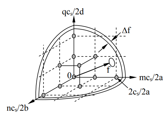
Each resonant mode A_mnq corresponds to one set of quantum numbers m,n,q and to one cell in the figure. Referring to (\ref{13.2.11}) it can be seen that frequency in the figure corresponds to the length of a vector from the origin to the mode A_mnq of interest. The total number N_o of acoustic modes with resonances at frequencies less than f_o is approximately the volume of the eighthsphere shown in the figure, divided by the volume of each cell of dimension (c_s/2a) × (c_s/2b) × (c_s/2d), where each cell corresponds to one acoustic mode. The approximation improves as f increases. Thus:

\[\mathrm{N}_{\mathrm{o}} \cong\left[4 \pi \mathrm{f}_{\mathrm{o}}^{3} /(3 \times 8)\right] /\left(\mathrm{c}_{\mathrm{s}}^{3} / 8 \mathrm{abd}\right)=4 \pi \mathrm{f}_{\mathrm{o}}^{3} \mathrm{V} / 3 \mathrm{c}_{\mathrm{s}}^{3} \ \ \left[\operatorname{modes}<\mathrm{f}_{\mathrm{o}}\right] \label{13.2.34}\]

In the electromagnetic case each set of quantum numbers m,n,q corresponds to both a TE and a TM resonant mode of a rectangular cavity, so N_o is then doubled:

\[{ }^{3} \mathrm{N}_{\mathrm{o}} \cong 8 \pi \mathrm{f}_{\mathrm{o}} \mathrm{V} / 3 \mathrm{C}^{2} \quad\left(\text { electromagnetic modes }<\mathrm{f}_{\mathrm{o}}\right) \label{13.2.35}\]

The number density n_o of acoustic modes per Hertz is the volume of a thin shell of thickness Δf, again divided by the volume of each cell:

\[\mathrm{n}_{\mathrm{o}} \cong \Delta \mathrm{f} \times 4 \pi \mathrm{f}^{2} /\left(8 \mathrm{c}_{\mathrm{s}}^{3} / 8 \mathrm{abd}\right)=\Delta \mathrm{f} 4 \pi \mathrm{f}^{2} \mathrm{V} / \mathrm{c}_{\mathrm{s}}^{3} \ \ \left[\operatorname{modes} \mathrm{Hz}^{-1}\right] \label{13.2.36}\]

Thus the modes of a resonator overlap more and tend to blend together as the frequency increases. The density of electromagnetic modes in a similar cavity is again twice that for acoustic modes.

Typical examples of acoustic resonators include musical instruments such as horns, woodwinds, organ pipes, and the human vocal tract. Rooms with reflective walls are another example. In each case if we wish to excite a particular mode efficiently the source must not only excite it with the desired frequency, but also from a favorable location.

One way to identify favorable locations for modal excitation is to assume the acoustic source exerts pressure p across a small aperture at the wall or interior of the resonator, and then to compute the incremental acoustic intensity transferred from that source to the resonator using (13.1.27):

\[\mathrm{I}=\mathrm{R}_{\mathrm{e}}\left\{\mathrm{pu}^{*} / 2\right\} \label{13.2.37}\]

In this expression we assume \( \overline{\mathrm{\underline u}}\) is dominated by waves already present in the resonator at the resonant frequency of interest and that the vector \( \overline{\mathrm{ u}}\) is normal to the surface across which p is applied. Therefore pressure sources located at velocity nulls for a particular mode transfer no power and no excitation occurs. Conversely, power transfer is maximized if pressure is applied at velocity maxima. Similarly, acoustic velocity sources are best located at a pressure maximum of a desired mode. For example, all acoustic modes have pressure maxima at the corners of rectangular rooms, so velocity loudspeakers located there excite all modes equally.

The converse is also true. If we wish to damp certain acoustic modes we may put absorber at their velocity or pressure maxima, depending on the type of absorber used. A wire mesh that introduces drag damps high velocities, and surfaces that reflect waves weakly (such as holes in pipes) damp pressure maxima. High frequency modes are more strongly damped in humid atmospheres than are low frequency modes, but such bulk absorption mechanisms do not otherwise discriminate among them.

Because the pressure and velocity maxima are located differently for each mode, each mode typically has a different Q, which is the number of radians before the total stored energy w_T decays by a factor of e^-1. Therefore the Q of any particular mode m,n,p is (7.4.34):

\[\mathrm{Q}=\omega_{\mathrm{o}} \mathrm{w}_{\mathrm{T}} / \mathrm{P}_{\mathrm{d}} \qquad \qquad \qquad \text{(acoustic Q)} \label{13.2.38}\]

The resonant frequencies and stored energies are given by (\ref{13.2.33}) and (13.1.25), respectively, where it suffices to compute either the maximum stored kinetic or potential energy, for they are equal. The power dissipated P_d can be found by integrating the intensity expression (\ref{13.2.37}) over the soft walls of the resonator, and adding any dissipation occurring in the interior.

Small changes in resonator shape can perturb acoustic resonant frequencies, much like electromagnetic resonances are perturbed. Whether a gentle indentation increases or lowers a particular resonant frequency depends on whether the time average acoustic pressure for the mode of interest is positive or negative at that indentation. It is useful to note that acoustic energy is quantized, where each phonon has energy hf Joules where h is Planck’s constant; this is directly analogous to a photon at frequency f. Therefore the total acoustic energy in a resonator at frequency f is:

\[\mathrm{w}_{\mathrm{T}}=\mathrm{nhf} \ [\mathrm{J}] \label{13.2.39}\]

If the cavity shape changes slowly relative to the frequency, the number n of acoustic phonons remains constant and any change in w_T results in a corresponding change in f. The work Δw_T done on the phonon field when cavity walls move inward Δz is positive if the time average acoustic pressure P_a is outward (positive), and negative if that pressure is inward or negative: Δw_T = P_aΔz. It is well known that gaseous flow parallel to a surface pulls on that surface as a result of the Bernoulli effect, which is the same effect that explains how airplane wings are supported in flight and how aspirators work. Therefore if an acoustic resonator is gently indented at a velocity maximum for a particular resonance, that resonant frequency f will be reduced slightly because the phonon field pulling the wall inward will have done work on the wall. All acoustic velocities at walls must be parallel to them. Conversely, if the indentation occurs near pressure maxima for a set of modes, the net acoustic force is outward and therefore the indentation does work on the phonon field, increasing the energy and frequency of those modes.

The most pervasive example of this phenomenon is human speech, which employs a vocal tract perhaps 16 cm long, typically less in women and all children. One end is excited by brief pulses in air pressure produced as the vocal chords vibrate at the pitch frequency of any vowel being uttered. The resulting train of periodic pressure pulses with period T has a frequency spectrum consisting of impulses spaced at T^-1 Hz, typically below 500 Hz. The vocal tract then accentuates those impulses falling near any resonance of that tract.

Figure \(\PageIndex{3}\): Acoustic resonances in tubes.

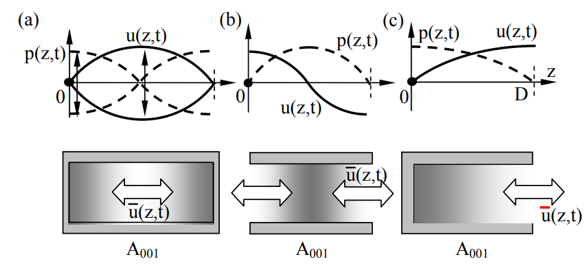
Figure 13.2.3 illustrates the lowest frequency acoustic resonances possible in pipes that are: (a) closed at both ends, (b) open at both ends, and (c) closed at one end and open at the other; each mode is designated A₀₀₁ for its own structure, where 00 corresponds to the fact that the acoustic wave is uniform in the x-y plane, and 1 indicates that it is the lowest non-zero-frequency resonant mode. Resonator (a) is capable of storing energy at zero frequency by pressurization (in the A₀₀₀ mode), and resonator (b) could store energy in the A₀₀₀ mode if there were a steady velocity in one direction through the structure; these A₀₀₀ modes are generally of no interest, and some experts do not consider them modes at all.

A sketch of the human vocal tract appears in Figure 13.2.4(a); at resonance it is generally open at the mouth and closed at the vocal chords, analogous to the resonator pictured in Figure 13.2.3(c). This structure resonates when its length D corresponds to one-quarter wavelength, three-quarters wavelength, or generally (2n-1)/4 wavelengths for the A_00n mode, as sketched in Figure 13.2.3(b). For a vocal tract 16 cm long and a velocity of sound c_s = 340 m s^-1, the lowest resonant frequency \(\mathrm{f_{001}=c_{s} / \lambda_{001}}=340 /(4 \times 0.16)=531 \ \mathrm{Hz}\). The next resonances, f₂ and f₃, fall at 1594 and 2656 Hz, respectively.

Figure \(\PageIndex{4}\): Human vocal tract.

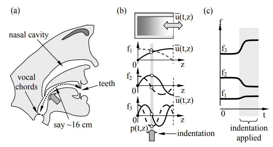
If the tongue now indents the vocal tract at the arrow indicated in (a) and (b) of Figure 13.2.4, then the three illustrated resonances will all shift as indicated in (c) of the figure. The resonance f₁ shifts only slightly upward because the indentation occurs between the peaks for velocity and pressure, but nearer to the pressure peak. The resonances shift more significantly down for f₂ and up for f₃ because this indentation occurs near velocity and pressure maximum for these two resonances, respectively, while occurring near a null for the complimentary variable. By simply controlling the width of the vocal tract at various positions using the tongue and teeth, these tract resonances can be modulated up and down to produce our full range of vowels.

These resonances are driven by periodic impulses of air released by the vocal cords at a pitch controlled by the speaker. The pitch is a fraction of the lowest vocal tract resonant frequency, and the impulses are sufficiently brief that their harmonics range up to 5 kHz and more. Speech also includes high-pitched broadband noise caused by turbulent air whistling past the teeth or other obstacles as in the consonants s, h, and f, and impulsive spikes caused by temporary tract closures, as in the consonants b, d, and p. Speech therefore includes both voiced (driven by vocal chord impulses) and unvoiced components. The spectral content of most consonants can similarly be modulated by the vocal tract and mouth.

It is possible to change the composition of the air in the vocal tract, thus altering the velocity of sound c_s and the resonant frequencies of the tract, which are proportional to c_s (\ref{13.2.30}). Thus when breathing helium all tract resonance frequencies increase by a noticeable fraction, equivalent to shortening the vocal tract. Note that pitch is not significantly altered by helium because the natural pitch of the vocal chords is determined instead primarily by their tension, composition, and length.