1.8: Flux

The product of electric field intensity and area is the flux $\Phi_E$. Whereas $E$ is an intensive quantity, $\Phi_E$ is an extensive quantity. It dimensions are ML³T^-2Q^-1 and its SI units are N m² C^-1, although later on, after we have met the unit called the volt, we shall prefer to express $\Phi_E$ in V m.

With increasing degrees of sophistication, flux may be defined mathematically as:

$$\Phi_E = EA$$

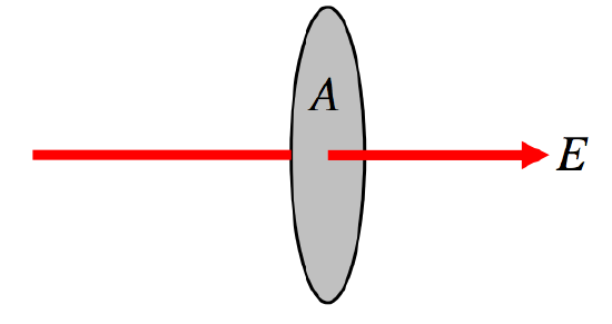
$\text{FIGURE I.4}$: Flow that is perpendicular to the surface.

$$\Phi_E = EA \cos \theta = \textbf{E} \cdot \textbf{A}$$

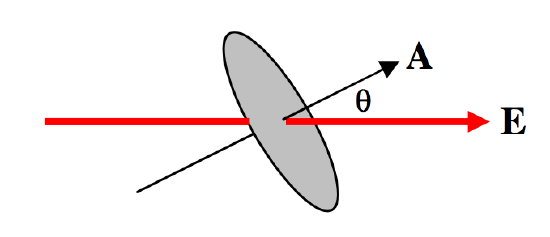
$\text{FIGURE I.5}$: Flow that is at an angle to the surface.

Note that $\textbf{E}$ is a vector, but $\Phi_E$ is a scalar.

$$\Phi_E = \iint \textbf{E} \cdot d\textbf{A}$$

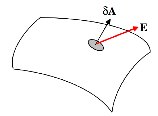
$\text{FIGURE I.6}$

We can also define a $D$-flux by

$$\Phi_D=\iint \textbf{D}\cdot d\textbf{A}.$$

The dimensions of $\Phi_D$ are just $Q$ and the SI units are coulombs (C).

An example is in order:

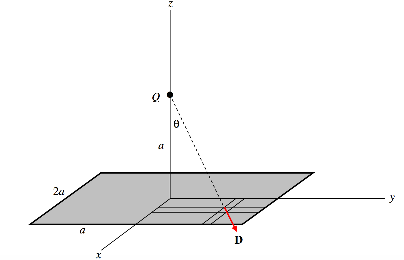
$\text{FIGURE I.7}$

Consider a square of side $2a$ in the xy-plane as shown. Suppose there is a positive charge $Q$ at a height $a$ on the $z$-axis. Calculate the total $D$-flux, $\Phi_D$ through the area.

Consider an elemental area $dxdy$ at ($x,\, y ,\, 0$). Its distance from $Q$ is $(a^2+x^2+y^2)^{1/2}$ so the magnitude of the $D$-field there is $\frac{Q}{4\pi}\cdot \frac{1}{a^2+x^2+y^2}$. The scalar product of this with the area is $\frac{Q}{4\pi}\cdot \frac{1}{a^2+x^2+y^2}\cdot \cos \theta dxdy,\text{ and }\cos \theta = \frac{a}{(a^2+x^2+y^2)^{1/2}}$. The surface integral of $\textbf{D}$ over the whole area is

$$\label{1.8.1}\iint D\cdot dA=\frac{Qa}{\pi}\int_0^a \int_0^a \frac{dxdy}{(a^2+x^2+y^2)^{3/2}}.$$

Now all we have to do is the nice and easy integral. Let $x=\sqrt{a^2+y^2}\tan ψ$ and the inner integral $\int_0^a \frac{dx}{(a^2+x^2+y^2)^{3/2}}$ reduces, after some modest algebra, to $\frac{a}{(a^2+y^2)\sqrt{2a^2+y^2}}$. Thus we now have

$$\label{1.8.2}\iint D\cdot dA = \frac{Qa^2}{\pi}\int_0^a \frac{dy}{(a^2+y^2)\sqrt{2a^2+y^2}}.$$

With the further substitution $a^2+y^2=a^2 \sec \omega$ this reduces, after more careful algebra, to

$$\iint D\cdot dA=\frac{Q}{6}.\label{1.8.3}$$

Two additional examples of calculating surface integrals may be found in Section 5.6, of the Celestial Mechanics section of these notes. These deal with gravitational fields, but they are essentially the same as the electrostatic case; just substitute $Q$ for m and -1/(4$\pi \epsilon$) for $G$.

I urge readers actually to go through the pain and the algebra and the trigonometry of these three examples in order that they may appreciate all the more, in the next section, the power of Gauss’s theorem.