Physics LibreTexts

6.6: Field on the Axis and in the Plane of a Plane Circular Current-carrying Coil

  • Page ID
    5450
  • \( \newcommand{\vecs}[1]{\overset { \scriptstyle \rightharpoonup} {\mathbf{#1}} } \) \( \newcommand{\vecd}[1]{\overset{-\!-\!\rightharpoonup}{\vphantom{a}\smash {#1}}} \)\(\newcommand{\id}{\mathrm{id}}\) \( \newcommand{\Span}{\mathrm{span}}\) \( \newcommand{\kernel}{\mathrm{null}\,}\) \( \newcommand{\range}{\mathrm{range}\,}\) \( \newcommand{\RealPart}{\mathrm{Re}}\) \( \newcommand{\ImaginaryPart}{\mathrm{Im}}\) \( \newcommand{\Argument}{\mathrm{Arg}}\) \( \newcommand{\norm}[1]{\| #1 \|}\) \( \newcommand{\inner}[2]{\langle #1, #2 \rangle}\) \( \newcommand{\Span}{\mathrm{span}}\) \(\newcommand{\id}{\mathrm{id}}\) \( \newcommand{\Span}{\mathrm{span}}\) \( \newcommand{\kernel}{\mathrm{null}\,}\) \( \newcommand{\range}{\mathrm{range}\,}\) \( \newcommand{\RealPart}{\mathrm{Re}}\) \( \newcommand{\ImaginaryPart}{\mathrm{Im}}\) \( \newcommand{\Argument}{\mathrm{Arg}}\) \( \newcommand{\norm}[1]{\| #1 \|}\) \( \newcommand{\inner}[2]{\langle #1, #2 \rangle}\) \( \newcommand{\Span}{\mathrm{span}}\)\(\newcommand{\AA}{\unicode[.8,0]{x212B}}\)

    I strongly recommend that you compare and contrast this derivation and the result with the treatment of the electric field on the axis of a charged ring in Section 1.6.4 of Chapter 1. Indeed I am copying the drawing from there and then modifying it as need be.
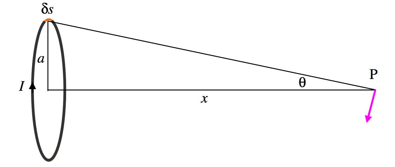
    VI.5.png
    \(\text{FIGURE VI.5}\)

    The contribution to the magnetic field at \(\text{P}\) from an element \(\delta s\) of the current is \(\dfrac{\mu I \delta s}{4\pi (a^2+x^2)}\) in the direction shown by the colored arrow. By symmetry, the total component of this from the entire coil perpendicular to the axis is zero, and the only component of interest is the component along the axis, which is \(\frac{\mu I \delta s}{4\pi (a^2+x^2)}\) times \(\sin \theta\).

    The integral of \(\delta s\) around the whole coil is just the circumference of the coil, \(2\pi a\), and if we write \(\sin \theta = \frac{a}{(a^2+x^2)^{1/2}},\) we find that the field at \(\text{P}\) from the entire coil is

    \[B=\dfrac{\mu I a^2}{2(a^2+x^2)^{3/2}},\]

    or \(N\) times this if there are \(N\) turns in the coil. At the centre of the coil the field is

    \[B=\dfrac{\mu I}{2a}.\]

    The field is greatest at the center of the coil and it decreases monotonically to zero at infinity. The field is directed to the left in Figure IV.5.

    We can calculate the field in the plane of the ring as follows.
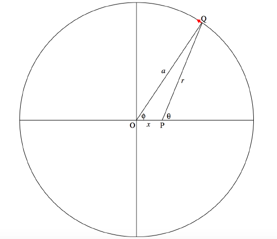
    VI. page 10.png

    Consider an element of the wire at \(\text{Q}\) of length \(ad\phi\). The angle between the current at \(\text{Q}\) and the line \(\text{PQ}\) is \(90^\circ - (\theta - \phi)\). The contribution to the \(B\)-field at \(\text{P}\) from the current \(I\) this element is

    \[\nonumber \frac{\mu_0}{4\pi}\cdot \frac{Ia\cos (\theta -\phi)\,d\phi}{r^2}.\]

    The field from the entire ring is therefore

    \[\frac{2\mu_0Ia}{4\pi}\int_0^\pi \frac{\cos (\theta -\phi)d\phi}{r^2},\nonumber\]

    where

    \[\nonumber r^2 = a^2+x^2 - 2ax\cos \phi,\]

    and

    \[\nonumber \cos (\theta -\phi) = \frac{a^2+r^2-x^2}{2ar}.\]

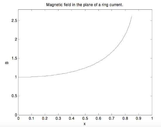
    This requires a numerical integration. The results are shown in the following graph, in which the abscissa, \(x\), is the distance from the center of the circle in units of its radius, and the ordinate, \(B\), is the magnetic field in units of its value \(\mu_0 I/(2a)\) at the center. Further out than \(x = 0.8\), the field increases rapidly.

    VI. page 11.png


    This page titled 6.6: Field on the Axis and in the Plane of a Plane Circular Current-carrying Coil is shared under a CC BY-NC 4.0 license and was authored, remixed, and/or curated by Jeremy Tatum via source content that was edited to the style and standards of the LibreTexts platform; a detailed edit history is available upon request.