8.5: Motion in a Nonuniform Magnetic Field

I give this as a rather more difficult example, not suitable for beginners, just to illustrate how one might calculate the motion of a charged particle in a magnetic field that is not uniform. I am going to suppose that we have an electric current $I$ flowing (in a wire) in the positive $z$-direction up the $z$-axis. An electron of mass $m$ and charge of magnitude $e$ (i.e., its charge is $−e$) is wandering around in the vicinity of the current. The current produces a magnetic field, and consequently the electron, when it moves, experiences a Lorenz force. In the following table I write, in cylindrical coordinates, the components of the magnetic field produced by the current, the components of the Lorentz force on the electron, and the expressions in cylindrical coordinates for acceleration component. Some facility in classical mechanics will be needed to follow this.

$$\begin{array}{c|lcr} & \text{Field} & \text{Force} & \text{Acceleration} \\ \hline \rho & B_\rho = 0 & e \dot z B_\phi & \ddot \rho - \rho \dot \phi^2 \\ \phi & B_\phi = \frac{\mu_0I}{2\pi\rho} & 0 & \rho \ddot \phi + 2 \dot\rho \dot\phi \\ z & B_z=0 & -e\dot\rho B_\phi & \ddot z \\ \nonumber \end{array}$$

From this table we can write down the equations of motion, as follows, in which $S_C$ is short for $\frac{\mu_0eI}{2\pi m}$. This quantity has the dimensions of speed (verify!) and I am going to call it the characteristic speed. It has the numerical value $3.5176 \times 10^4 \text{I m s}^{−1}$, where $I$ is in $A$. The equations of motion, then, are

Radial:

$$\rho(\ddot \rho - \rho \dot\phi^2) =S_C \dot z$$

Transverse (Azimuthal):

$$\rho \ddot \phi + 2 \dot \rho \dot \phi = 0$$

Longitudinal:

$$\rho \ddot z = -S_C \dot \rho .$$

It will be convenient to define dimensionless velocity components:

$$u=\dot\rho/S_C, \qquad v= \rho \dot\phi/S_C, \qquad w=\dot z /S_c .\label{8.5.4a,b,c}$$

Suppose that initially, at time $t = 0$, their values are $u_0$, $v_0$ and $w_0$, and also that the initial distance of the particle from the current is $\rho_0$. Further, introduce the dimensionless distance

$$x=\rho/\rho_0,$$

so that the initial value of $x$ is 1. The initial values of $\phi$ and $z$ may be taken to be zero by suitable choice of axes.

Integration of equations 8.5.2 and 3, with these initial conditions, yields

$$\dot z = S_C(w_0 - \ln (\rho/\rho_0))$$

and

$$\rho^2 \dot \phi = \rho_0 v_0 S_C;$$

or, in terms of the dimensionless variables,

$$w=w_0-\ln x$$

and

$$v=v_0/x.$$

We may write $\dot\rho \frac{d\dot\rho}{d\rho}$ for $\ddot\rho$ in equation 8.5.1, and substitution for $\dot z$ and $\dot\phi$ from equations 8.5.6 and 8.5.7 yields

$$u^2=u_0^2+v_0^2(1-1/x^2) + 2 w_0 \ln x - (\ln x)^2.$$

Equations 8.5.8,9 and 10 give the velocity components of the electron as a function of its distance from the wire.

Equation 8.5.2 expresses the fact that there is no transverse (azimuthal) force. Its time integral, equation 8.5.7) expresses the consequence that the $z$-component of its angular momentum is conserved. Further, from equations 8.5.8,9 and 10, we find that

$$u^2 +v^2 + w^2 = u_0^2 +v_0^2 +w_0^2 =s^2,\ \text{say},$$

so that the speed of the electron is constant. This is as expected, since the force on the electron is always perpendicular to its velocity; the point of application of the force does not move in the direction of the force, which therefore does no work, so that kinetic energy, and hence speed, is conserved.

The distance of the electron from the wire is bounded below and above. The lower and upper bounds, $x_1$ and $x_2$ are found from equation 8.5.10 by putting $u = 0$ and solving for $x$. Examples of these bounds are shown in the Table $\text{VIII.I}$ for a variety of initial conditions.

$\text{TABLE VII.1}$

$\text{BOUNDS OF THE MOTION}$

$$\begin{array}{c\qquad c\qquad l\qquad c\qquad r} |u_0| & |v_0| & |w_0| & x_1 & x_2 \\ 0 & 0 & −2 & 0.018 & 1.000 \\ 0 & 0 & −1 & 0.135 & 1.000 \\ 0 & 0 & 0 & 1.000 & 1.000 \\ 0 & 0 & 1 & 1.000 & 7.389 \\ 0 & 0 & 2 & 1.000 & 54.598 \\ 0 & 1 & −2 & 0.599 & 1.000 \\ 0 & 1 & −1 & 1.000 & 1.000 \\ 0 & 1 & 0 & 1.000 & 2.501 \\ 0 & 1 & 1 & 1.000 & 11.149 \\ 0 & 1 & 2 & 1.000 & 69.132 \\ 0 & 2 & −2 & 1.000 & 1.845 \\ 0 & 2 & −1 & 1.000 & 3.137 \\ 0 & 2 & 0 & 1.000 & 7.249 \\ 0 & 2 & 1 & 1.000 & 25.398 \\ 0 & 2 & 2 & 1.000 & 125.009 \\ 1 & 0 & −2 & 0.014 & 1.266 \\ 1 & 0 & −1 & 0.089 & 1.513 \\ 1 & 0 & 0 & 0.368 & 2.718 \\ 1 & 0 & 1 & 0.661 & 11.181 \\ 1 & 0 & 2 & 0.790 & 69.135 \\ 1 & 1 & −2 & 0.476 & 1.412 \\ 1 & 1 & −1 & 0.602 & 1.919 \\ 1 & 1 & 0 & 0.726 & 4.024 \\ 1 & 1 & 1 & 0.809 & 15.345 \\ 1 & 1 & 2 & 0.857 & 85.581 \\ 1 & 2 & −2 & 0.840 & 2.420 \\ 1 & 2 & −1 & 0.873 & 4.052 \\ 1 & 2 & 0 & 0.896 & 9.259 \\ 1 & 2 & 1 & 0.912 & 31.458 \\ 1 & 2 & 2 & 0.925 & 148.409 \\ 2 & 0 & −2 & 0.008 & 2.290 \\ 2 & 0 & −1 & 0.039 & 3.442 \\ 2 & 0 & 0 & 0.135 & 7.389 \\ 2 & 0 & 1 & 0.291 & 25.433 \\ 2 & 0 & 2 & 0.437 & 125.014 \\ 2 & 1 & −2 & 0.352 & 2.654 \\ 2 & 1 & −1 & 0.409 & 4.212 \\ 2 & 1 & 0 & 0.474 & 9.332 \\ 2 & 1 & 1 & 0.542 & 31.478 \\ 2 & 1 & 2 & 0.605 & 148.412 \\ 2 & 2 & −2 & 0.647 & 4.183 \\ 2 & 2 & −1 & 0.681 & 7.297 \\ 2 & 2 & 0 & 0.712 & 16.877 \\ 2 & 2 & 1 & 0.740 & 54.486 \\ 2 & 2 & 2 & 0.764 & 236.061 \\ \nonumber \end{array}$$

In analysing the motion in more detail, we can start with some particular initial conditions. One easy case is if $u_0 = v_0 = w_0 = 0$ – i.e. the electron starts at rest. In that case there will be no forces on it, and it remains at rest for all time. A less trivial initial condition is for $v_0 = 0$, but the other components not zero. In that case, equation 8.5.7 shows that $\phi$ is constant for all time. What this means is that the motion all takes place in a plane $\phi = \text{constant}$, and there is no motion “around” the wire. This is just to be expected, because the $\rho$-component of the velocity gives rise to a $z$-component of the Lorenz force, and the $z$-component of the velocity gives rise to a Lorentz force towards the wire, and there is no component of force “around” (increasing $\phi$) the wire. The electron, then, is going to move in the plane $\phi = \text{constant}$ at a constant speed $S=sS_C$, where $s=\sqrt{u_0^2+w_0^2}$. (Recall that $u$ and $w$ are dimensionless quantities, being the velocity components in units of the characteristic speed $S_C.$) I am going to coin the words perineme and aponeme to describe the least and greatest distances of the electrons from the wire – i.e. the bounds of the motion. These bounds can be found by setting $u = 0$ and $v_0 = 0$ in equation 8.5.10 (where we recall that $x = \rho/\rho_0$ - i.e. the ratio of the radial distance of the electron at some time to its initial radial distance). We obtain

$$\rho=\rho_0e^{w_0 \pm s}$$

for the aponeme (upper sign) and perineme (lower sign) distances. From equation 8.5.8 we can deduce that the electron is moving at right angles to the wire (i.e. $w = 0$) when it is at a distance

$$\rho = \rho_0e^{w_0}.$$

The form of the trajectory with v0 = 0 is found by integrating equations 8.5.8 and 8.5.10. It is convenient to start the integration at perineme so that u0 = 0 and s = w0, and the initial value of x ( / ) = ρ ρ0 is 1. For any other initial conditions, the perineme values of x and ρ can be found from equations 8.5.10 and 8.5.12 respectively. Equations 8.5.10 and 8.5.8 may them be written

$$t=\frac{\rho_0}{S_C} \int_1^x \frac{dx}{[2s \ln x - (\ln x)^2]^{1/2}}$$

and

$$z= St-\rho_0 \int_1^x \frac{\ln x dx}{[2s \ln x - (\ln x )^2]^{1/2}}.$$

There are singularities in the integrands at $x = 1$ and $\ln x = 2s$, and, in order to circumvent this difficulty it is convenient to introduce a variable $\theta$ defined by

$$\ln x = s(1-\sin \theta).$$

Equations 8.5.14 and 15 then become

$$t=\frac{\rho_0e^s}{S_C}\int_{\pi/2}^0 e^{-s \sin \theta} d\theta$$

and

$$z=\rho_0 se^s \int_{\pi/2}^0 \sin \theta e^{-s\sin\theta} d\theta.$$

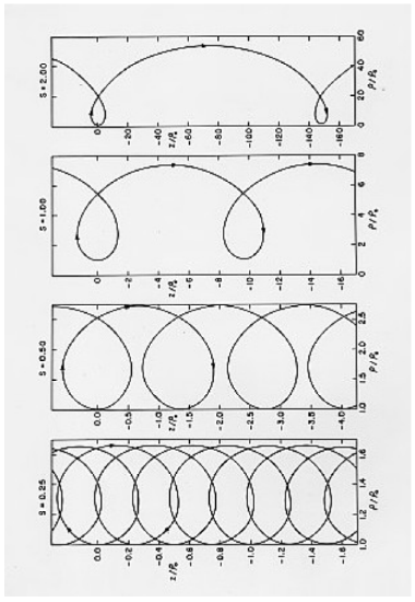
Examples of these trajectories are shown in Figure $\text{VIII.4}$, though I’m afraid you will have to turn your monitor on its side to view it properly. They are drawn for $s =$ 0.25, 0.50, 1.00 and 2.00, where $s$ is the ration of the constant electron speed to the characteristic speed $S_C$. The wire is supposed to be situated along the $z$-axis ($\rho = 0$) with the current flowing in the direction of positive $z$. The electron drifts in the opposite direction to the current. (A positively charged particle would drift in the same direction as the current.) Distances in the Figure are expressed in terms of the perineme distance $\rho_0$. The shape of the path depends only on $s$ (and not on $\rho$). For no speed does the path have a cusp. The radius of curvature $R$ at any point is given by $R = \rho/s$.

Minima of $\rho$ occur at $\rho_0$ and $\theta = (4n + 1)\pi/2$, where $n$ is an integer;

Maxima of $z$ occur at $\rho = \rho_0 e^s$ and $\theta = (4n + 2)\pi/2$ ;

Maxima of $\rho$ occur at $\rho = \rho_0e^{2s}$ and $\theta = (4n + 3)\pi/2$ ;

Minima of $z$ occur at $\rho = \rho_0e^s$ and $\theta = (4n + 4)\pi/2$.

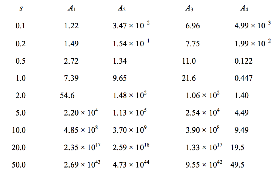
The distance between successive loops and the period of each loop vary rapidly with electron speed, as is illustrated in Table $\text{VIII.2}$. In this table, $s$ is the electron speed in units of the characteristic speed $S_C$, $A_1$ is the ratio of aponeme to perineme distance, $A_2$ is the ratio of interloop distance to perineme distance, $A_3$ is the ratio of period per loop to $\rho_0/S_C$, and $A_4$ is the drift speed in units of the characteristic speed $S_C$.

$\text{FIGURE VIII.4}$

For example, for a current of 1 $\text{A}$, the characteristic speed is $3.5176 \times 10^4 \text{m s}^{−1}$. If an electron is accelerated through $8.7940 \text{V}$, it will gain a speed of $1.7588 \text{m s}^{−1}$, which is 50 times the characteristic speed. If the electron starts off at this speed moving in the same direction as the current and $10^{-10}$ from it, it will reach a maximum distance of $8.72 \times 10^{10}$ megaparsecs ( 1 $\text{Mpc} = 3.09 \times 10^{22} \text{m}$) from it, provided the Universe is euclidean. The distance between the loops will be $1.53 \times 10^{12} \text{Mpc}$, and the period will be $8.60 \times 10^{20}$ years, after which the electron will have covered, at constant speed, a total distance of $1.55 \times 10^{12} \text{Mpc}$. The drift speed will be $1.741 \times 10^6 \text{m s}^{−1}$.

$\text{TABLE VIII.2}$

Let us now turn to consideration of cases where $v_0 \neq 0$ so that the motion of the electron is not restricted to a plane. At first glance is might be thought that since an azimuthal velocity component gives rise to no additional Lorenz force on the electron, the motion will hardly be affected by a nonzero $v_0$, other than perhaps by a revolution around the wire. In particular, for given initial velocity components $u_0$ and $w_0$, the perineme and aponeme distances $x_1$ and $x_2$ might seem to be independent of $v_0$. Reference to Table $\text{VIII.1}$, however, shows that this is by no means so. The reason is that as the electron moves closer to or further from the wire, the changes in $v$ made necessary by conservation of the $z$-component of the angular momentum are compensated for by corresponding changes in $u$ and $w$ made necessary by conservation of kinetic energy.

Since the motion is bounded above and below, there will always be some time when $\dot \rho = 0$. There is no loss of generality if we shift the time origin so as to choose $\dot \rho = 0$ when $t = 0$ and $x = 1$. From this point, therefore, we shall consider only those trajectories for which $u_0 = 0$. In other words we shall follow the motion from a time $t = 0$ when the electron is at an apsis ($\dot\rho = 0$). [The plural of apsis is apsides. The word apse (plural apses) is often used in this connection, but it seems useful to maintain a distinction between the architectural term apse and the mathematical term apsis.] Whether this apsis is perineme (so that $\dot\rho= \rho_1$, $v_0 =v_1$, $w_0=w_1$) or aponeme (so that $\dot\rho = \rho_2$, $v_0 =v_2$, $w_0=w_2$) depends on the subsequent motion.

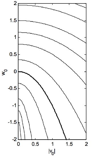
The electron starts, then, at a distance from the wire defined by $x = 1$. It is of interest to find the value of $x$ at the next apsis, in terms of the initial velocity components $v_0$ and $w_0$. This is found from equation 8.5.10 with $u = 0$ and $u_0 = 0$. The results are shown in Figure $\text{VIII.5}$. This Figure shows loci of constant next apsis distance, for values of $x$ (going from bottom left to top right of the Figure) of 0.05, 0.10, 0.20, 0.50, 1, 2, 5, 10, 20, 50, 100. The heavy curve is for $x = 1$. It will immediately be seen that, if $w_0 > -v_0^2$, (above the heavy curve) the value of $x$ at the second apsis is greater than 1. (Recall that $v$ and $w$ are dimensionless ratios, so there is no problem of dimensional imbalance in the inequality.) The electron was therefore initially at perineme and subsequently moves away from the wire. If on the other hand , $w_0 < -v_0^2$, (below the heavy curve) the value of $x$ at the second apsis is less than 1. The electron was therefore initially at aponeme and subsequently moves closer to the wire.

$\text{FIGURE VIII.5}$

The case where $w_0 = -v_0^2$ is of special interest, for them perineme and aponeme distances are equal and indeed the electron stays at a constant distance from the wire at all times. It moves in a helical trajectory drifting in the opposite direction to the direction of the conventional current $I$. (A positively charged particle would drift in the same direction as $I$.) The pitch angle $\alpha$ of the helix (i.e. the angle between the instantaneous velocity and a plane normal to the wire) is given by

$$\tan\alpha = -w/v,$$

where $w$ and $v$ are constrained by the equations

$$w_0 = -v_0^2$$

and

$$v^2 + w^2 = s^2.$$

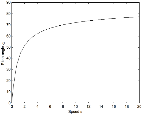
This implies that the pitch angle is determined solely by $s$, the ratio of the speed $S$ of the electron to the characteristic speed $S_C$. On other words, the pitch angle is determined by the ratio of the electron speed $S$ to the current $I$. The variation of pitch angle $\alpha$ with speed $s$ is shown in Figure $\text{VIII.6}$. This relation is entirely independent of the radius of the helix.

$\text{FIGURE VIII.6}$

If , $w_o \neq -v_0^2$ the electron no longer moves in a simple helix, and the motion must be calculated numerically for each case. It is convenient to start the calculation at perineme with initial conditions $u_0=0$, $w_0 > -v_0^2$, $x_0=1$. For other initial conditions, the perineme (and aponeme) values of $u$, $v$, $w$ and $\rho$ can easily be found from equations 8.5.10 (with $u_0 = 0$), 8.5.8 and 8.5.9. Starting, then, from perineme, integrations of these equations take the respective forms

$$t=\frac{\rho_0}{S_C}\int^x_1[v_0^2(1-1/x^2)+2w_0\ln x -(\ln x )^2 ]^{-1/2}dx,$$

and

$$z=w_0S_Ct-\rho_0 \int^x_1v_0^2(1-1/x^2) + 2w_0 \ln x - (\ln x)^2]^{-1/2} \ln x \ dx$$

$$\phi =v_0 \int^x_1 [v_0^2(1-1/x^2) + 2w_0 \ln x - (\ln x )^2]^{-1/2}x^{-2}\ dx.$$

The integration of these equations is not quite trivial and is discussed in the Appendix (Section 8A).

In general the motion of the electron can be described qualitatively roughly as follows. The motion is bounded between two cylinders of radii equal to the perineme and aponeme distances, and the speed is constant. The electron moves around the wire in either a clockwise or a counterclockwise direction, but, once started, the sense of this motion does not change. The angular speed around the wire is greatest at perineme and least at aponeme, being inversely proportional to the square of the distance from the wire. Superimposed on the motion around the wire is a general drift in the opposite direction to that of the conventional current. However, for a brief moment near perineme the electron is temporarily moving in the same direction as the current.

An example of the motion is given in Figures $\text{VIII.7}$ and 8 for initial velocity components $u_0 = 0$, $v_0 = w_0 = 1$. The aponeme distance is 11.15 times the perineme distance. The time interval between two perineme passages is 26.47 $\rho_0/S_C$. The time interval for a complete revolution around the wire ($\phi = 360^\circ$ ) is 68.05 $\rho_0/S_C$. In Figure $\text{VIII.8}$, the conventional electric current is supposed to be flowing into the plane of the “paper” (computer screen), away from the reader. The portions of the electron trajectory where the electron is moving towards from the reader are drawn as a continuous line, and the brief portions near perineme where the electron is moving away from the reader are indicated by a dotted line. Time marks on the Figure are at intervals of $5\rho_0/S_C$.

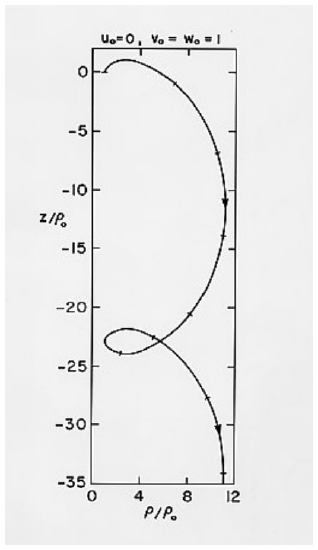
$\text{FIGURE VIII.7}$

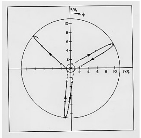
$\text{FIGURE VIII.8}$