12.6: Ferromagnetism
- Page ID
- 5492
\( \newcommand{\vecs}[1]{\overset { \scriptstyle \rightharpoonup} {\mathbf{#1}} } \)
\( \newcommand{\vecd}[1]{\overset{-\!-\!\rightharpoonup}{\vphantom{a}\smash {#1}}} \)
\( \newcommand{\dsum}{\displaystyle\sum\limits} \)
\( \newcommand{\dint}{\displaystyle\int\limits} \)
\( \newcommand{\dlim}{\displaystyle\lim\limits} \)
\( \newcommand{\id}{\mathrm{id}}\) \( \newcommand{\Span}{\mathrm{span}}\)
( \newcommand{\kernel}{\mathrm{null}\,}\) \( \newcommand{\range}{\mathrm{range}\,}\)
\( \newcommand{\RealPart}{\mathrm{Re}}\) \( \newcommand{\ImaginaryPart}{\mathrm{Im}}\)
\( \newcommand{\Argument}{\mathrm{Arg}}\) \( \newcommand{\norm}[1]{\| #1 \|}\)
\( \newcommand{\inner}[2]{\langle #1, #2 \rangle}\)
\( \newcommand{\Span}{\mathrm{span}}\)
\( \newcommand{\id}{\mathrm{id}}\)
\( \newcommand{\Span}{\mathrm{span}}\)
\( \newcommand{\kernel}{\mathrm{null}\,}\)
\( \newcommand{\range}{\mathrm{range}\,}\)
\( \newcommand{\RealPart}{\mathrm{Re}}\)
\( \newcommand{\ImaginaryPart}{\mathrm{Im}}\)
\( \newcommand{\Argument}{\mathrm{Arg}}\)
\( \newcommand{\norm}[1]{\| #1 \|}\)
\( \newcommand{\inner}[2]{\langle #1, #2 \rangle}\)
\( \newcommand{\Span}{\mathrm{span}}\) \( \newcommand{\AA}{\unicode[.8,0]{x212B}}\)
\( \newcommand{\vectorA}[1]{\vec{#1}} % arrow\)
\( \newcommand{\vectorAt}[1]{\vec{\text{#1}}} % arrow\)
\( \newcommand{\vectorB}[1]{\overset { \scriptstyle \rightharpoonup} {\mathbf{#1}} } \)
\( \newcommand{\vectorC}[1]{\textbf{#1}} \)
\( \newcommand{\vectorD}[1]{\overrightarrow{#1}} \)
\( \newcommand{\vectorDt}[1]{\overrightarrow{\text{#1}}} \)
\( \newcommand{\vectE}[1]{\overset{-\!-\!\rightharpoonup}{\vphantom{a}\smash{\mathbf {#1}}}} \)
\( \newcommand{\vecs}[1]{\overset { \scriptstyle \rightharpoonup} {\mathbf{#1}} } \)
\(\newcommand{\longvect}{\overrightarrow}\)
\( \newcommand{\vecd}[1]{\overset{-\!-\!\rightharpoonup}{\vphantom{a}\smash {#1}}} \)
\(\newcommand{\avec}{\mathbf a}\) \(\newcommand{\bvec}{\mathbf b}\) \(\newcommand{\cvec}{\mathbf c}\) \(\newcommand{\dvec}{\mathbf d}\) \(\newcommand{\dtil}{\widetilde{\mathbf d}}\) \(\newcommand{\evec}{\mathbf e}\) \(\newcommand{\fvec}{\mathbf f}\) \(\newcommand{\nvec}{\mathbf n}\) \(\newcommand{\pvec}{\mathbf p}\) \(\newcommand{\qvec}{\mathbf q}\) \(\newcommand{\svec}{\mathbf s}\) \(\newcommand{\tvec}{\mathbf t}\) \(\newcommand{\uvec}{\mathbf u}\) \(\newcommand{\vvec}{\mathbf v}\) \(\newcommand{\wvec}{\mathbf w}\) \(\newcommand{\xvec}{\mathbf x}\) \(\newcommand{\yvec}{\mathbf y}\) \(\newcommand{\zvec}{\mathbf z}\) \(\newcommand{\rvec}{\mathbf r}\) \(\newcommand{\mvec}{\mathbf m}\) \(\newcommand{\zerovec}{\mathbf 0}\) \(\newcommand{\onevec}{\mathbf 1}\) \(\newcommand{\real}{\mathbb R}\) \(\newcommand{\twovec}[2]{\left[\begin{array}{r}#1 \\ #2 \end{array}\right]}\) \(\newcommand{\ctwovec}[2]{\left[\begin{array}{c}#1 \\ #2 \end{array}\right]}\) \(\newcommand{\threevec}[3]{\left[\begin{array}{r}#1 \\ #2 \\ #3 \end{array}\right]}\) \(\newcommand{\cthreevec}[3]{\left[\begin{array}{c}#1 \\ #2 \\ #3 \end{array}\right]}\) \(\newcommand{\fourvec}[4]{\left[\begin{array}{r}#1 \\ #2 \\ #3 \\ #4 \end{array}\right]}\) \(\newcommand{\cfourvec}[4]{\left[\begin{array}{c}#1 \\ #2 \\ #3 \\ #4 \end{array}\right]}\) \(\newcommand{\fivevec}[5]{\left[\begin{array}{r}#1 \\ #2 \\ #3 \\ #4 \\ #5 \\ \end{array}\right]}\) \(\newcommand{\cfivevec}[5]{\left[\begin{array}{c}#1 \\ #2 \\ #3 \\ #4 \\ #5 \\ \end{array}\right]}\) \(\newcommand{\mattwo}[4]{\left[\begin{array}{rr}#1 \amp #2 \\ #3 \amp #4 \\ \end{array}\right]}\) \(\newcommand{\laspan}[1]{\text{Span}\{#1\}}\) \(\newcommand{\bcal}{\cal B}\) \(\newcommand{\ccal}{\cal C}\) \(\newcommand{\scal}{\cal S}\) \(\newcommand{\wcal}{\cal W}\) \(\newcommand{\ecal}{\cal E}\) \(\newcommand{\coords}[2]{\left\{#1\right\}_{#2}}\) \(\newcommand{\gray}[1]{\color{gray}{#1}}\) \(\newcommand{\lgray}[1]{\color{lightgray}{#1}}\) \(\newcommand{\rank}{\operatorname{rank}}\) \(\newcommand{\row}{\text{Row}}\) \(\newcommand{\col}{\text{Col}}\) \(\renewcommand{\row}{\text{Row}}\) \(\newcommand{\nul}{\text{Nul}}\) \(\newcommand{\var}{\text{Var}}\) \(\newcommand{\corr}{\text{corr}}\) \(\newcommand{\len}[1]{\left|#1\right|}\) \(\newcommand{\bbar}{\overline{\bvec}}\) \(\newcommand{\bhat}{\widehat{\bvec}}\) \(\newcommand{\bperp}{\bvec^\perp}\) \(\newcommand{\xhat}{\widehat{\xvec}}\) \(\newcommand{\vhat}{\widehat{\vvec}}\) \(\newcommand{\uhat}{\widehat{\uvec}}\) \(\newcommand{\what}{\widehat{\wvec}}\) \(\newcommand{\Sighat}{\widehat{\Sigma}}\) \(\newcommand{\lt}{<}\) \(\newcommand{\gt}{>}\) \(\newcommand{\amp}{&}\) \(\definecolor{fillinmathshade}{gray}{0.9}\)What we normally think of as magnetic materials are technically ferromagnetic. The susceptibilities of ferromagnetic materials are typically of order +103 or 104 or even greater. However, the ferromagnetic susceptibility of a material is quite temperature sensitive, and, above a temperature known as the Curie temperature, the material ceases to become ferromagnetic, and it becomes merely paramagnetic.
Among the elements, only cobalt, iron and nickel are strongly ferromagnetic, their Curie temperatures being about 1400, 1040 and 630 K respectively. Gadolinium is ferromagnetic at low temperatures; its Curie temperature is about 289 K = 16 oC. Dysprosium is ferromagnetic below its Curie temperature of about 105 K. There are many artificial alloys and ceramic materials which are ferromagnetic.
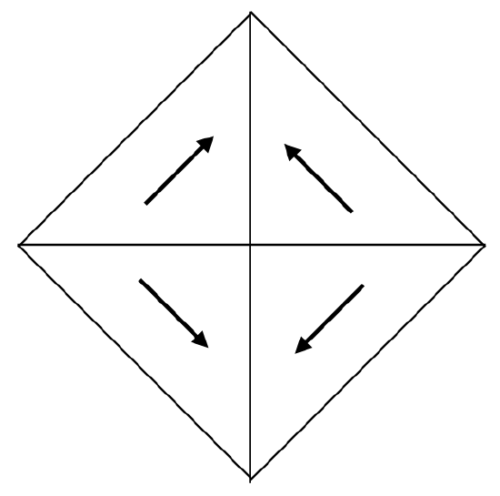
As with paramagnetic materials, the atoms have permanent magnetic moments, but with the difference that these moments are not randomly oriented but are strongly aligned to the crystallographic axes. Within a single crystal, there exist domains, within which all the magnetic moments are parallel and are aligned with a particular axis. In an adjacent domain, again all the moments are parallel to each other, but they may be aligned with a different axis, perhaps at right angles to the first domain, or perhaps aligned with the same axis but pointing in the opposite direction. Thus we have a number of domains, each highly magnetized, but with some domains magnetized in one direction and some in another. The domains are separated by domain boundaries, or “Bloch walls”, perhaps a few hundred atoms thick, within which the orientation of the magnetic moments gradually changes from one domain to the next. Figure XII.1 is a schematic sketch of a crystal divided into four domains, with the magnetization in a different direction in each.

Figure XIII.1
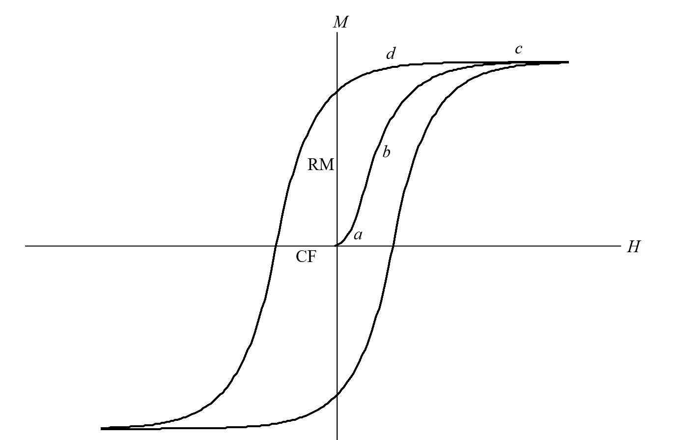
In Figure XIII.2 I am exposing the crystal to a progressively stronger and stronger magnetic field, and we watch what happens to the domains, and, in Figure XIII.3, to the magnetization of the crystal as a whole.

Figure XIII.2
When we first apply a weak field (a), the Bloch walls (domain boundaries) move so that the favorably-oriented domains grow at the expense of the opposing domains, and the magnetization slowly increases. With stronger fields (b), suddenly all the magnetic moments (due to unpaired spins) within a single domain change direction almost in unison, so that an opposing domain suddenly becomes a favorable domain; this happens to one domain after another, until all domains are oriented favorably, and the magnetization of the specimen rapidly increases. For yet stronger fields (c), the magnetic moments, usually oriented parallel to a crystal axis, bend so that they are in the direction of the magnetizing field. When all of that is achieved, no further magnetization is possible, and the specimen is saturated.

Figure XIII.3
Now, if the field is reduced, the magnetic moments relax and take up their normal positions parallel to a crystallographic axis. But, as the field is further reduced (d), there is no reason for the domains to reverse their polarity as happened at stage (b). That is, when stage (b) originally happened, this was an irreversible process. The demagnetization curve does not follow the magnetization curve in reverse. Consequently, when the magnetizing field has been reduced to zero, the specimen retains a remanent magnetization (indicated by RM in Figure XIII.3), with all domains still favorably oriented. In order to reduce the magnetization to zero, you have to apply a field in the reverse direction. The reverse field needed to reduce the magnetization to zero is called the coercive force (indicated by CF in Figure XIII.3).
As you repeatedly magnetize the specimen first on one direction and then the other, the graph of magnetization versus magnetizing field describes the hysteresis loop indicated in Figure XII.3. Because of the irreversible process (b), magnetic energy is dissipated as heat during a complete cycle, the about of energy loss being proportional to the area of the hysteresis loop. The amount of the hysteresis depends on how freely the domain walls can move, which in turn depends on the physical and chemical constitution of the magnetic materials, particularly on the number of impurities present that can inhibit Bloch wall movement. For a permanent magnet, you need a material with a fat hysteresis loop, with a large remanent magnetization as well as a large coercive force, so that it cannot be demagnetized easily. For a transformer core, you need a material with a narrow hysteresis loop.
If you put a magnetic material inside a solenoid with alternating current inside the solenoid, the magnetization will repeatedly go around the hysteresis loop. If you now gradually decrease the amplitude of the current in the solenoid, the hysteresis loop will gradually become smaller and smaller, vanishing to a point (H and M both zero) when the current is reduced to zero. This provides a method of demagnetizing a specimen.
It is distressing how often one reads of the “remnant” magnetization. I have even encountered over-enthusiastic copy-editors who will change an author’s correct spelling “remanent” to the incorrect “remnant”. The difference is that “remnant” is a noun (as in a remnant of cloth) and “remanent”, which is pronounced with three distinct syllables, is an adjective, meaning “remaining”.


