8.2: Acceptance Angle

In this section, we consider the problem of injecting light into a fiber optic cable. The problem is illustrated in Figure \(\PageIndex{1}\).

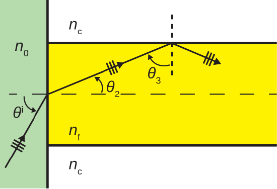Figure \(\PageIndex{1}\): Injecting light into a fiber optic cable. ( CC BY-SA 4.0; S. Lally)

In this figure, we see light incident from a medium having index of refraction \(n_0\), with angle of incidence \(\theta^i\). The light is transmitted with angle of transmission \(\theta_2\) into the fiber, and is subsequently incident on the surface of the cladding with angle of incidence \(\theta_3\). For light to propagate without loss within the cable, it is required that

\[\sin\theta_3 \ge \frac{n_c}{n_f} \label{m0192_eCAnm} \]

since this criterion must be met in order for total internal reflection to occur.

Now consider the constraint that Equation \ref{m0192_eCAnm} imposes on \(\theta^i\). First, we note that \(\theta_3\) is related to \(\theta_2\) as follows:

\[\theta_3 = \frac{\pi}{2} - \theta_2 \nonumber \]

therefore

\begin{align} \sin\theta_3 &= \sin\left(\frac{\pi}{2} - \theta_2\right) \\ &= \cos\theta_2 \end{align}

so

\[\cos\theta_2 \ge \frac{n_c}{n_f} \nonumber \]

Squaring both sides, we find:

\[\cos^2\theta_2 \ge \frac{n_c^2}{n_f^2} \nonumber \]

Now invoking a trigonometric identity:

\[1-\sin^2\theta_2 \ge \frac{n_c^2}{n_f^2} \nonumber \]

so:

\[\sin^2\theta_2 \le 1-\frac{n_c^2}{n_f^2} \label{m0192_e1} \]

Now we relate the \(\theta_2\) to \(\theta^i\) using Snell’s law:

\[\sin\theta_2 = \frac{n_0}{n_f}\sin\theta^i \nonumber \]

so Equation \ref{m0192_e1} may be written:

\[\frac{n_0^2}{n_f^2}\sin^2\theta^i \le 1-\frac{n_c^2}{n_f^2} \nonumber \]

Now solving for \(\sin\theta^i\), we obtain:

\[\sin\theta^i \le \frac{1}{n_0}\sqrt{ n_f^2 - n_c^2 } \nonumber \]

This result indicates the range of angles of incidence which result in total internal reflection within the fiber. The maximum value of \(\theta^i\) which satisfies this condition is known as the acceptance angle \(\theta_a\), so:

\[\theta_a \triangleq \arcsin\left(\frac{1}{n_0}\sqrt{ n_f^2 - n_c^2 }\right) \nonumber \]

This leads to the following insight:

In order to effectively launch light in the fiber, it is necessary for the light to arrive from within a cone having half-angle \(\theta_a\) with respect to the axis of the fiber.

The associated cone of acceptance is illustrated in Figure \(\PageIndex{2}\).

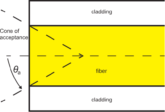Figure \(\PageIndex{2}\): Cone of acceptance. ( CC BY-SA 4.0)

It is also common to define the quantity numerical aperture NA as follows:

\[\mbox{NA} \triangleq \frac{1}{n_0}\sqrt{ n_f^2 - n_c^2 } \label{m0192_eNA} \]

Note that \(n_0\) is typically very close to \(1\) (corresponding to incidence from air), so it is common to see NA defined as simply \(\sqrt{ n_f^2 - n_c^2 }\). This parameter is commonly used in lieu of the acceptance angle in datasheets for fiber optic cable.

Example \(\PageIndex{1}\): Acceptance angle

Typical values of \(n_f\) and \(n_c\) for an optical fiber are 1.52 and 1.49, respectively. What are the numerical aperture and the acceptance angle?

Solution

Using Equation \ref{m0192_eNA} and presuming \(n_0=1\), we find NA \(\cong \underline{0.30}\). Since \(\sin\theta_a =\) NA, we find \(\theta_a=\underline{17.5^{\circ}}\). Light must arrive from within \(17.5^{\circ}\) from the axis of the fiber in order to ensure total internal reflection within the fiber.