5.4: Magnetic Dipole Moment and Magnetic Dipole Media

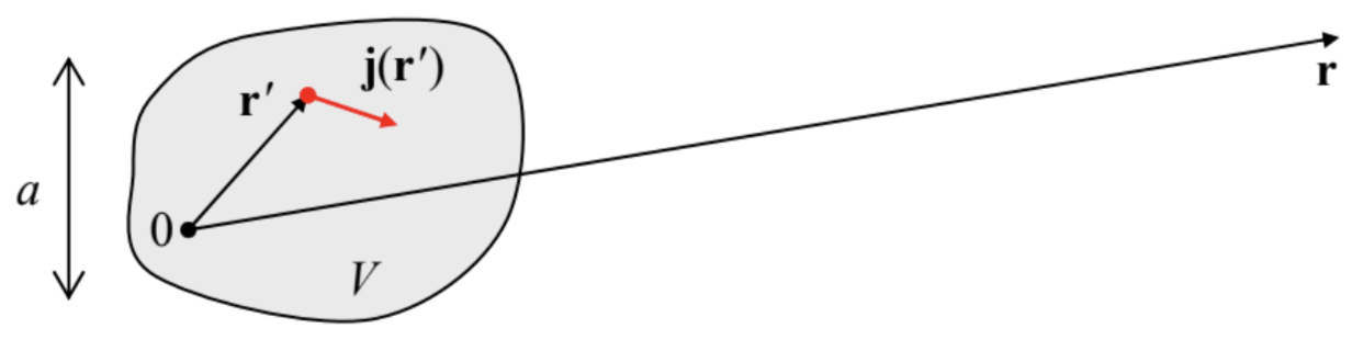
The most natural way of the magnetic media description parallels that described in Chapter 3 for dielectrics, and is based on properties of magnetic dipoles – the notion close (but not identical!) to that of the electric dipoles discussed in Sec. 3.1. To introduce this notion quantitatively, let us consider, just as in Sec. 3.1, a spatially-localized system with a current distribution \(\ \mathbf{j}\left(\mathbf{r}^{\prime}\right)\), whose magnetic field is measured at relatively large distances \(\ r >> r^{\prime}\) (Fig. 10).

Fig. 5.10. Calculating the magnetic field of localized currents at a distant point \(\ (r>>a)\).

Applying the truncated Taylor expansion (3.5) of the fraction \(\ 1 /\left|\mathbf{r}-\mathbf{r}^{\prime}\right|\) to the vector potential given by Eq. (28), we get

\[\ \mathbf{A}(\mathbf{r}) \approx \frac{\mu_{0}}{4 \pi}\left[\frac{1}{r} \int_{V} \mathbf{j}\left(\mathbf{r}^{\prime}\right) d^{3} r^{\prime}+\frac{1}{r^{3}} \int_{V}\left(\mathbf{r} \cdot \mathbf{r}^{\prime}\right) \mathbf{j}\left(\mathbf{r}^{\prime}\right) d^{3} r^{\prime}\right].\tag{5.84}\]

Now, due to the vector character of this potential, we have to depart slightly from the approach of Sec. 3.1 and use the following vector algebra identity:³⁹

\[\ \int_{V}[f(\mathbf{j} \cdot \nabla g)+g(\mathbf{j} \cdot \nabla f)] d^{3} r=0,\tag{5.85}\]

that is valid for any pair of smooth (differentiable) scalar functions \(\ f(\mathbf{r})\) and \(\ g(\mathbf{r})\), and any vector function \(\ \mathbf{j}(\mathbf{r})\) that, as the dc current density, satisfies the continuity condition \(\ \nabla \cdot \mathbf{j}=0\) and whose normal component vanishes on the surface of the volume \(\ V\). First, let us use Eq. (85) with \(\ f\) equal to 1, and \(\ g\) equal to any Cartesian component of the radius-vector \(\ \mathbf{r}\): \(\ g=r_{l}(l=1,2,3)\). Then it yields

\[\ \int_{V}\left(\mathbf{j} \cdot \mathbf{n}_{l}\right) d^{3} r=\int_{V} j_{l} d^{3} r=0,\tag{5.86}\]

so that for the vector as the whole

\[\ \int_{V} \mathbf{j}(\mathbf{r}) d^{3} r=0,\tag{5.87}\]

showing that the first term on the right-hand side of Eq. (84) equals zero. Next, let us use Eq. (85) again, now with \(\ f=r_{l}, g=r_{l’}\left(l, l^{\prime}=1,2,3\right)\); then it yields

\[\ \int_{V}\left(r_{l} j_{l^{\prime}}+r_{l^{\prime}} j_{l}\right) d^{3} r=0,\tag{5.88}\]

so that the \(\ l^{\text {th }}\) Cartesian component of the second integral in Eq. (84) may be transformed as

\[\ \begin{aligned}
\int_{V}\left(\mathbf{r} \cdot \mathbf{r}^{\prime}\right) j_{l} d^{3} r^{\prime} &=\int_{V} \sum_{l^{\prime}=1}^{3} r_{l’} r_{l’}^{\prime} j_{l} d^{3} r^{\prime}=\frac{1}{2} \sum_{l^{\prime}=1}^{3} r_{l^{\prime}} \int_{V}\left(r_{l^{\prime}}^{\prime} j_{l}+r_{l^{\prime}}^{\prime} j_{l}\right) d^{3} r^{\prime} \\
&=\frac{1}{2} \sum_{l^{\prime}=1}^{3} r_{l^{\prime}} \int_{V}\left(r_{l^{\prime}}^{\prime} j_{l}-r_{l^{\prime}}^{\prime} j_{l^{\prime}}\right) d^{3} r^{\prime}=-\frac{1}{2}\left[\mathbf{r} \times \int_{V}\left(\mathbf{r}^{\prime} \times \mathbf{j}\right) d^{3} r^{\prime}\right]_{l}.
\end{aligned}\tag{5.89}\]

As a result, Eq. (84) may be rewritten as

Magnetic dipole and its potential

\[\ \mathbf{A}(\mathbf{r})=\frac{\mu_{0}}{4 \pi} \frac{\mathbf{m} \times \mathbf{r}}{r^{3}},\tag{5.90}\]

where the vector \(\ \mathbf{m}\), defined as⁴⁰

\[\ \mathbf{m} \equiv \frac{1}{2} \int_{V} \mathbf{r} \times \mathbf{j}(\mathbf{r}) d^{3} r,\tag{5.91}\]

is called the magnetic dipole moment of the system – that itself, within the long-rang approximation (90), is called the magnetic dipole.

Note a close analogy between the \(\ \mathbf{m}\) defined by Eq. (91), and the orbital⁴¹ angular momentum of a non-relativistic particle with mass \(\ m_{k}\):

\[\ \mathbf{L}_{k} \equiv \mathbf{r}_{k} \times \mathbf{p}_{k}=\mathbf{r}_{k} \times m_{k} \mathbf{V}_{k},\tag{5.92}\]

where \(\ \mathbf{p}_{k}=m_{k} \mathbf{v}_{k}\) is its linear momentum. Indeed, for a continuum of such particles with equal electric charges \(\ q\), distributed with spatial density \(\ n\), we have \(\ \mathbf{j}=q n \mathbf{v}\), and Eq. (91) yields

\[\ \mathbf{m}=\int_{V} \frac{1}{2} \mathbf{r} \times \mathbf{j} d^{3} r=\int_{V} \frac{n q}{2} \mathbf{r} \times \mathbf{v} d^{3} r,\tag{5.93}\]

while the total angular momentum of such a system of particles of equal masses \(\ m_{0}\), is

\(\ \mathbf{L}=\int_{V} n m_{0} \mathbf{r} \times \mathbf{v} d^{3} r,\)

so that we get a very straightforward relation

\[\ \mathbf{m}=\frac{q}{2 m_{0}} \mathbf{L}. \quad\quad\quad\quad\text{m vs. L}\tag{5.95}\]

For the orbital motion, this classical relation survives in quantum mechanics for linear operators, and hence for eigenvalues of the observables. Since the orbital angular momentum is quantized in the units of the Planck’s constant \(\ \hbar\), the orbital magnetic moment of an electron is always a multiple of the so-called Bohr magneton

\[\ \mu_{\mathrm{B}} \equiv \frac{e \hbar}{2 m_{\mathrm{e}}}\quad\quad\quad\quad\text{Bohr magneton}\tag{5.96}\]

where \(\ m_{\mathrm{e}}\) is the free electron mass.⁴² However, for particles with spin, such a universal relation between the vectors \(\ \mathbf{m}\) and \(\ \mathbf{L}\) is no longer valid. For example, the electron’s spin \(\ s=1 / 2\) gives a contribution of \(\ \hbar / 2\) to its mechanical angular momentum, but a contribution still very close to \(\ \mu_{\mathrm{B}}\) to its magnetic moment.

The next important example of a magnetic dipole is a planar thin-wire loop, limiting area \(\ A\) (of arbitrary shape), and carrying current \(\ I\), for which \(\ \mathbf{m}\) has a surprisingly simple form,

\[\ \mathbf{m}=I \mathbf{A},\tag{5.97}\]

where the modulus of the vector \(\ \mathbf{A}\) equals the loop’s area \(\ A\), and its direction is normal to the loop’s plane. This formula may be readily proved by noticing that if we select the coordinate origin on the plane of the loop (Fig. 11), then the elementary component of the magnitude of the integral (91),

\[\ d m=\frac{1}{2}\left|\oint_{C} \mathbf{r} \times I d \mathbf{r}\right| \equiv I \oint_{C}\left|\frac{1}{2} \mathbf{r} \times d \mathbf{r}\right|=I \oint_{C} \frac{1}{2} r^{2} d \varphi,\tag{5.98}\]

is just the elementary area \(\ d A=(1 / 2) r d(r \varphi)=r^{2} d \varphi / 2\) – the equality already used in CM Eq. (3.40).

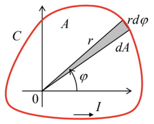Fig. 5.11. Calculating the magnetic dipole moment of a planar current loop.

The combination of Eqs. (96) and (97) allows a useful estimate of the scale of atomic currents, by finding what current \(\ I\) should flow in a circular loop of the atomic size scale (the Bohr radius) \(\ r_{\mathrm{B}} \sim 0.5\times10^{-10} \mathrm{m}\), i.e. of an area \(\ A \sim 10^{-20} \mathrm{~m}^{2}\), to produce a magnetic moment of the order of \(\ \mu_{\mathrm{B}}\).⁴³ The result is surprisingly macroscopic: \(\ I \sim 1 \mathrm{~mA}\) – quite comparable to the currents driving the sound in your phone’s earbuds. Though this estimate should not be taken too literally, due to the quantum-mechanical spread of electron's wavefunctions, it is very useful for getting a feeling of how significant the atomic magnetism is, and hence why ferromagnets may provide such strong magnetic fields.

After these illustrations, let us return to the discussion of the general Eq. (90). Plugging it into (also general) Eq. (27), we may calculate the magnetic field of a magnetic dipole: ⁴⁴

\[\ \mathbf{B}(\mathbf{r})=\frac{\mu_{0}}{4 \pi} \frac{3 \mathbf{r}(\mathbf{r} \cdot \mathbf{m})-\mathbf{m} r^{2}}{r^{5}}.\quad\quad\quad\quad\text{Magnetic dipole’s field}\tag{5.99}\]

The structure of this formula exactly replicates that of Eq. (3.13) for the electric dipole field – including the sign). Because of this similarity, the energy of a dipole of a fixed magnitude m in an external field, and hence the torque and the force exerted on it by a fixed external field, are given by expressions fully similar to those for an electric dipole – see Eqs. (3.15)-(3.19):⁴⁵

\[\ U=-\mathbf{m} \cdot \mathbf{B}_{\mathrm{ext}},\quad\quad\quad\quad\text{Magnetic dipole in external field}\tag{5.100}\]

and as a result,

\[\ \boldsymbol{\tau}=\mathbf{m} \times \mathbf{B}_{\mathrm{ext}},\tag{5.101}\]

\[\ \mathbf{F}=\nabla\left(\mathbf{m} \cdot \mathbf{B}_{\mathrm{ext}}\right).\tag{5.102}\]

Now let us consider a system of many magnetic dipoles (e.g., atoms or molecules), distributed in space with an atomic-scale-averaged density \(\ n\). Now let us consider a system of many magnetic dipoles (e.g., atoms or molecules), distributed in space with an atomic-scale-averaged density n. Then we can use Eq. (90), generalized in an evident way for an arbitrary position \(\ \mathbf{r}^{\prime}\) of the dipole, and the linear superposition principle, to calculate the macroscopic vector potential \(\ \mathbf{A}\):

\[\ \mathbf{A}(\mathbf{r})=\frac{\mu_{0}}{4 \pi} \int \frac{\mathbf{M}\left(\mathbf{r}^{\prime}\right) \times\left(\mathbf{r}-\mathbf{r}^{\prime}\right)}{\left|\mathbf{r}-\mathbf{r}^{\prime}\right|^{3}} d^{3} r^{\prime},\tag{5.103}\]

where \(\ \mathbf{M} \equiv n \mathbf{m}\) is the magnetization: the average magnetic moment per unit volume. Transforming this integral absolutely similarly to how Eq. (3.27) had been transformed into Eq. (3.29), we get:

\[\ \mathbf{A}(\mathbf{r})=\frac{\mu_{0}}{4 \pi} \int \frac{\nabla^{\prime} \times \mathbf{M}\left(\mathbf{r}^{\prime}\right)}{\left|\mathbf{r}-\mathbf{r}^{\prime}\right|} d^{3} r^{\prime}.\tag{5.104}\]

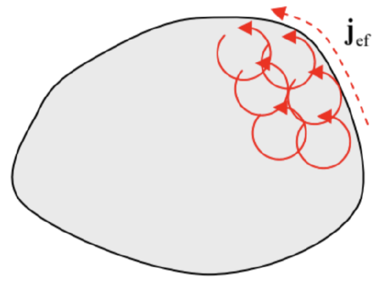
Comparing this result with Eq. (28), we see that \(\ \boldsymbol{\nabla} \times \mathbf{M}\) is equivalent, in its magnetic effect, to the density \(\ \mathbf{j}_{e f}\) of a certain effective “magnetization current”. Just as the electric-polarization charge \(\ \rho_{\mathrm{ef}}\) discussed in Sec. 3.2 (see Fig. 3.4), the vector \(\ \mathbf{j}_{\mathrm{ef}}=\nabla \times \mathbf{M}\) may be interpreted as the uncompensated part of the loop currents representing single magnetic dipoles \(\ \mathbf{m}\) (Fig. 12). Note, however, that since the atomic dipoles may be due to particles’ spins, rather than the actual electric currents due to the orbital motion, the magnetization current’s nature is not as direct as that of the polarization charge.

Now, using Eq. (28) to add the possible contribution from stand-alone currents \(\ \mathbf{j}\), not included into the currents of microscopic magnetic dipoles, we get the general expression for the vector potential of the macroscopic field:

\[\ \mathbf{A}(\mathbf{r})=\frac{\mu_{0}}{4 \pi} \int \frac{\left[\mathbf{j}\left(\mathbf{r}^{\prime}\right)+\nabla^{\prime} \times \mathbf{M}\left(\mathbf{r}^{\prime}\right)\right]}{\left|\mathbf{r}-\mathbf{r}^{\prime}\right|} d^{3} r^{\prime}.\tag{5.105}\]

Repeating the calculations that have led us from Eq. (28) to the Maxwell equation (35), with the account of the magnetization current term, for the macroscopic magnetic field \(\ \mathbf{B}\) we get

\[\ \nabla \times \mathbf{B}=\mu_{0}(\mathbf{j}+\nabla \times \mathbf{M}).\tag{5.106}\]

Fig. 5.12. A cartoon illustrating the physical nature of the effective magnetization current \(\ \mathbf{j}_{\text {ef }}=\nabla \times \mathbf{M}\).

Following the same reasoning as in Sec. 3.2, we may recast this equation as

\[\ \nabla \times \mathbf{H}=\mathbf{j},\tag{5.107}\]

where the field defined as

\[\ \text{Magnetic field H}\quad\quad\quad\quad\mathbf{H} \equiv \frac{\mathbf{B}}{\mu_{0}}-\mathbf{M},\tag{5.108}\]

by historic reasons (and very unfortunately) is also called the magnetic field.⁴⁶ This is why it is crucial to remember that the physical sense of field \(\ \mathbf{H}\) is very much different from field \(\ \mathbf{B}\). In order to understand this difference better, let us use Eq. (107) to bring Eqs. (3.32), (3.36), (29) and (107) together, writing them as the following system of macroscopic Maxwell equations (again, so far for the stationary case \(\ \partial / \partial t=0\)):⁴⁷

\[\ \text{Stationary macroscopic Maxwell equations}\quad\quad\quad\quad\begin{array}{ll}
\nabla \times \mathbf{E}=0, & \nabla \times \mathbf{H}=\mathbf{j}, \\
\nabla \cdot \mathbf{D}=\rho, & \nabla \cdot \mathbf{B}=0.
\end{array}\tag{5.109}\]

These equations clearly show that the roles of vector fields \(\ \mathbf{D}\) and \(\ \mathbf{H}\) are very similar: they both may be called “would-be fields” – the fields that would be induced by the stand-alone charges \(\ \rho\) and currents \(\ \mathbf{j}\), if the medium had not modified them by its dielectric and magnetic polarization.

Despite this similarity, let me note an important difference of signs in the relation (3.33) between \(\ \mathbf{E}\), \(\ \mathbf{D}\), and \(\ \mathbf{P}\), on one hand, and the relation (108) between \(\ \mathbf{B}\), \(\ \mathbf{H}\), and \(\ \mathbf{M}\), on the other hand. This is not just a matter of definition. Indeed, due to the similarity of Eqs. (3.15) and (100), including similar signs, the electric and magnetic fields both try to orient the corresponding dipole moments along the field. Hence, in the media that allow such an orientation (and as we will see momentarily, for magnetic media it is not always the case), the induced polarizations \(\ \mathbf{P}\) and \(\ \mathbf{M}\) are directed along, respectively, the vectors \(\ \mathbf{E}\) and \(\ \mathbf{B}\) of the genuine (though macroscopic, i.e. atomic-scale-averaged) fields. According to Eq. (3.33),
if the would-be field \(\ \mathbf{D}\) is fixed – say, by a fixed stand-alone charge distribution \(\ \rho(\mathbf{r})\) – such a polarization reduces the electric field \(\ \mathbf{E}=(\mathbf{D}-\mathbf{P}) / \varepsilon_{0}\). On the other hand, Eq. (108) shows that in a magnetic media with a fixed would-be field \(\ \mathbf{H}\), the magnetic polarization making \(\ \mathbf{M}\) parallel to \(\ \mathbf{B}\), enhances the magnetic field \(\ \mathbf{B}=\mu_{0}(\mathbf{H}+\mathbf{M})\). This difference may be traced back to the sign difference in the basic relations (1) and (2), i.e. to the fundamental fact that the electric charges of the same sign repulse, while the currents of the same direction attract each other.

---

Reference

³⁹ See, e.g., MA Eq. (12.3) with the additional condition \(\ \left.j_{n}\right|_{S}=0\), pertinent to space-restricted currents.

⁴⁰ In the Gaussian units, the definition (91) is kept valid, so that Eq. (90) is stripped of the factor \(\ \mu_{0} / 4 \pi\).

⁴¹ This adjective is used, especially in quantum mechanics, to distinguish the motion of a particle as a whole (not necessarily along a closed orbit!) from its intrinsic angular momentum, the spin – see, e.g., QM Chapters 3-6.

⁴² In the SI units, \(\ m_{\mathrm{e}} \approx 0.91 \times 10^{-30} \mathrm{~kg}\), so that \(\ \mu_{\mathrm{B}} \approx 0.93 \times 10^{-23} \mathrm{~J} / \mathrm{T}\).

⁴³ Another way to arrive at the same estimate is to take \(\ I \sim e f=e \omega / 2 \pi\) with \(\ \omega \sim 10^{16} \mathrm{~s}^{-1}\) being the typical frequency of radiation due to atomic interlevel quantum transitions.

⁴⁴ Similarly to the situation with the electric dipoles (see Eq. (3.24) and its discussion), it may be shown that the magnetic field of any closed current loop (or any system of such loops) satisfies the following equality:

\(\ \int_{V} \mathbf{B}(\mathbf{r}) d^{3} r=(2 / 3) \mu_{0} \mathbf{m},\)

where the integral is over any sphere confining all the currents. On the other hand, as we know from Sec. 3.1, for a field with the structure (99), derived from the long-range approximation (90), such an integral vanishes. As a result, to get a coarse-grain description of the magnetic field of a small system, located at \(\ r = 0\), which would give the correct average value of the magnetic field, Eq. (99) should be modified as follows:

\(\ \mathbf{B}_{\mathrm{cg}}(\mathbf{r})=\frac{\mu_{0}}{4 \pi}\left(\frac{3 \mathbf{r}(\mathbf{r} \cdot \mathbf{m})-\mathbf{m} r^{2}}{r^{5}}+\frac{8 \pi}{3} \mathbf{m} \delta(\mathbf{r})\right),\)

in a conceptual (though not quantitative) similarity to Eq. (3.25).

⁴⁵ Note that the fixation of \(\ m\) and \(\ \mathbf{B}_{\mathrm{ext}}\) effectively means that the currents producing them are fixed – please have one more look at Eqs. (35) and (97). As a result, Eq. (100) is a particular case of Eq. (53) rather than (54) – hence the minus sign.

⁴⁶ This confusion is exacerbated by the fact that in Gaussian units, Eq. (108) has the form \(\ \mathbf{H}=\mathbf{B}-4 \pi \mathbf{M}\), and hence the fields \(\ \mathbf{B}\) and \(\ \mathbf{H}\) have the same dimensionality (and are formally equal in free space!) – though the unit of \(\ \mathbf{H}\) has a different name (oersted, abbreviated as Oe). Mercifully, in the SI units, the dimensionality of \(\ \mathbf{B}\) and \(\ \mathbf{H}\) is different, with the unit of \(\ \mathbf{H}\) called the ampere per meter.

⁴⁷ Let me remind the reader once again that in contrast with the system (36) of the Maxwell equations for the genuine (microscopic) fields, the right-hand sides of Eqs. (109) represent only the stand-alone charges and currents, not included in the microscopic electric and magnetic dipoles.