6.6: Inductors, Transformers, and AC Kirchhoff Laws

Let a wire coil (meaning either a single loop illustrated in Fig. 5.4b or a series of such loops, such as one of the solenoids shown in Fig. 5.6) have a self-inductance \(\ L\) much larger than that of the wires connecting it to other components of our system: ac voltage sources, voltmeters, etc. (Since, according to Eq. (5.75), \(\ L\) scales as the square of the number \(\ N\) of wire turns, this condition is easier to satisfy at \(\ N >>1\).) Then in a quasistatic system consisting of such lumped induction coils and external wires (and other lumped circuit elements such as resistors, capacitances, etc.), we may neglect the electromagnetic induction effects everywhere outside the coil, so that the electric field in those external regions is potential. Then the voltage V between coil’s terminals may be defined (as in electrostatics) as the difference of values of \(\ \phi\) between the terminals, i.e. as the integral

\[\ V=\int \mathbf{E} \cdot d \mathbf{r}\tag{6.83}\]

between the coil terminals along any path outside the coil. This voltage has to be balanced by the induction e.m.f. (2) in the coil, so that if the Ohmic resistance of the coil is negligible, we may write

\[\ V=\frac{d \Phi}{d t},\tag{6.84}\]

where \(\ \Phi\) is the magnetic flux in the coil.⁵³ If the flux is due to the current \(\ I\) in the same coil only (i.e. if it is magnetically uncoupled from other coils), we may use Eq. (5.70) to get the well-known relation

\[\ \text{Voltage drop on inductance coil}\quad\quad\quad\quad V=L \frac{d I}{d t},\tag{6.85}\]

where the compliance with the Lenz sign rule is achieved by selecting the relations between the assumed voltage polarity and the current direction as shown in Fig. 8a.

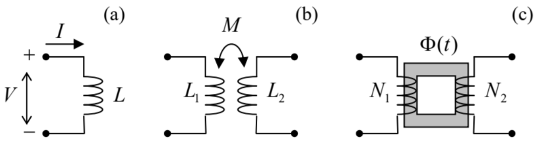Fig. 6.8. Some lumped ac circuit elements: (a) an induction coil, (b) two inductively coupled coils, and (c) an ac transformer.

If similar conditions are satisfied for two magnetically coupled coils (Fig. 8b), then, in Eq. (84), we need to use Eqs. (5.69) instead, getting

\[\ V_{1}=L_{1} \frac{d I_{1}}{d t}+M \frac{d I_{2}}{d t}, \quad V_{2}=L_{2} \frac{d I_{2}}{d t}+M \frac{d I_{1}}{d t}.\tag{6.86}\]

Such systems of inductively coupled coils have numerous applications in electrical engineering and physical experiment. Perhaps the most important of them is the ac transformer, in which the coils share a common soft-ferromagnetic core of the toroidal (“doughnut”) topology – see Fig. 8c.⁵⁴ As we already know from the discussion in Sec. 5.6, such cores, with \(\ \mu>>\mu_{0}\), “try” to absorb all magnetic field lines, so that the magnetic flux \(\ \Phi(t)\) in the core is nearly the same in each of its cross sections. With this, Eq. (84) yields

\[\ V_{1} \approx N_{1} \frac{d \Phi}{d t}, \quad V_{2} \approx N_{2} \frac{d \Phi}{d t},\tag{6.87}\]

so that the voltage ratio is completely determined by the ratio \(\ N_{1} / N_{2}\) of the number of wire turns.

Now we may generalize, to the ac current case, the Kirchhoff laws already discussed in Chapter 4 – see Fig. 4.3 reproduced in Fig. 9a below. Let not only inductances but also capacitances and resistances of the wires be negligible in comparison with those of the lumped (compact) circuit elements, whose list now would include not only resistors and current sources (as in the dc case), but also the induction coils (including magnetically coupled ones) and capacitors – see Fig. 9b. In the quasistatic approximation, the current flowing in each wire is conserved, so that the “node rule”, i.e. the 1^st Kirchhoff law (4.7a),

\[\ \sum_{j} I_{j}=0.\tag{6.88a}\]

remains valid. Also, if the electromagnetic induction effect is restricted to the interior of lumped induction coils as discussed above, the voltage drops \(\ V_{k}\) across each circuit element may be still represented, just as in dc circuits, with differences of potentials of the adjacent nodes. As a result, the “loop rule”, i.e. 2^nd Kirchhoff law (4.7b),

\[\ \sum_{k} V_{k}=0,\tag{6.88b}\]

is also valid. In contrast to the dc case, Eqs. (88) are now the (ordinary) differential equations. However, if all circuit elements are linear (as in the examples presented in Fig. 9b), these equations may be readily reduced to linear algebraic equations, using the Fourier expansion. (In the common case of sinusoidal ac sources, the final stage of the Fourier series summation is unnecessary.)

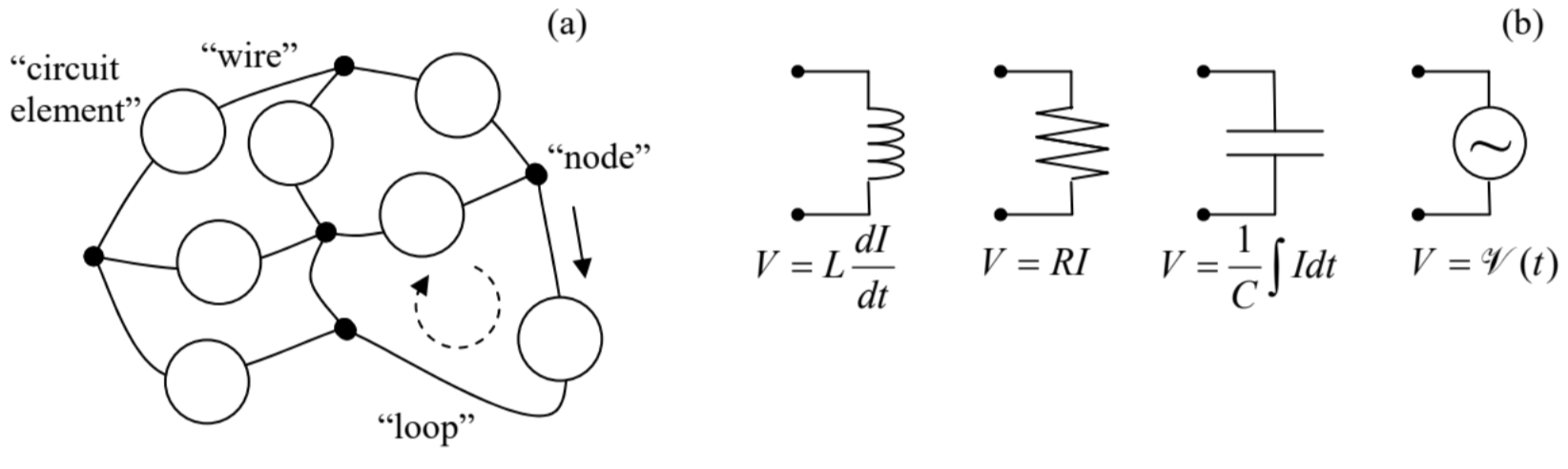Fig. 6.9. (a) A typical quasistatic ac circuit obeying the Kirchhoff laws, and (b) the simplest lumped circuit elements.

My teaching experience shows that the potential readers of these notes are well familiar with the application of Eqs. (88) to such problems from their undergraduate studies, so I would like to save time/space by skipping discussions of even the simplest examples of such circuits, such as \(\ LC\), \(\ LR\), \(\ RC\), and \(\ LRC\) loops and periodic structures.⁵⁵ However, since these problems are very important for practice, my sincere advice to the reader is to carry out a self-test by solving a few problems of this type,
provided at the end of this chapter, and if they cause any difficulty, go after some remedial reading.

---

Reference

⁵³ If the resistance is substantial, it may be represented by a separate lumped circuit element (resistor) connected in series with the coil.

⁵⁴ The first practically acceptable form of this device, called the Stanley transformer, in which multi-turn windings could be easily mounted onto a toroidal ferromagnetic (at that time, silicon-steel-plate) core, was invented in 1886.

⁵⁵ Curiously enough, these effects include wave propagation in periodic LC circuits, even within the quasistatic approximation! However, the speed \(\ 1 /(L C)^{1 / 2}\) of these waves in lumped circuits is much lower than the speed \(\ 1 /(\varepsilon \mu)^{1 / 2}\) of electromagnetic waves in the surrounding medium – see Sec. 8 below.