6.9: Exercise Problems

Last updated
Save as PDF

Page ID: 57011

\( \newcommand{\vecs}[1]{\overset { \scriptstyle \rightharpoonup} {\mathbf{#1}} } \) \( \newcommand{\vecd}[1]{\overset{-\!-\!\rightharpoonup}{\vphantom{a}\smash {#1}}} \)\(\newcommand{\id}{\mathrm{id}}\) \( \newcommand{\Span}{\mathrm{span}}\) \( \newcommand{\kernel}{\mathrm{null}\,}\) \( \newcommand{\range}{\mathrm{range}\,}\) \( \newcommand{\RealPart}{\mathrm{Re}}\) \( \newcommand{\ImaginaryPart}{\mathrm{Im}}\) \( \newcommand{\Argument}{\mathrm{Arg}}\) \( \newcommand{\norm}[1]{\| #1 \|}\) \( \newcommand{\inner}[2]{\langle #1, #2 \rangle}\) \( \newcommand{\Span}{\mathrm{span}}\) \(\newcommand{\id}{\mathrm{id}}\) \( \newcommand{\Span}{\mathrm{span}}\) \( \newcommand{\kernel}{\mathrm{null}\,}\) \( \newcommand{\range}{\mathrm{range}\,}\) \( \newcommand{\RealPart}{\mathrm{Re}}\) \( \newcommand{\ImaginaryPart}{\mathrm{Im}}\) \( \newcommand{\Argument}{\mathrm{Arg}}\) \( \newcommand{\norm}[1]{\| #1 \|}\) \( \newcommand{\inner}[2]{\langle #1, #2 \rangle}\) \( \newcommand{\Span}{\mathrm{span}}\)\(\newcommand{\AA}{\unicode[.8,0]{x212B}}\)

6.1. Prove that the electromagnetic induction e.m.f. \(\ \mathscr{V}_{\text {ind }}\) in a conducting loop may be measured as shown on two panels of Fig. 1:

(i) by measuring the current \(\ I=\mathscr{V}_{\mathrm{ind}} / R\) induced in the loop closed with an Ohmic resistor \(\ R\), or

(ii) using a voltmeter inserted into the loop.

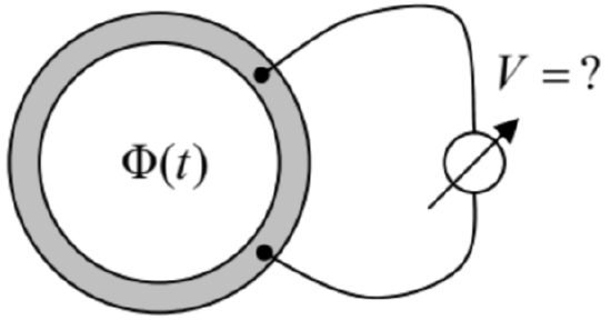
6.2. The flux \(\ \Phi\) of the magnetic field that pierces a resistive ring is being changed in time, while the magnetic field outside of the ring is negligibly low. A voltmeter is connected to a part of the ring, as shown in the figure on the right. What would the voltmeter show?

Screen Shot 2022-02-13 at 10.47.52 PM.png

6.3. A weak, uniform magnetic field \(\ \mathbf{B}\) is applied to an axially-symmetric permanent magnet, with the dipole magnetic moment \(\ \mathbf{m}\) directed along the symmetry axis, rapidly rotating about the same axis, with an angular momentum \(\ \mathbf{L}\). Calculate the electric field resulting from the magnetic field’s
application, and formulate the conditions of your result’s validity.

6.4. The similarity of Eq. (5.53), obtained in Sec. 5.3 without any use of the Faraday induction law, and Eq. (5.54), proved in Sec. 2 of this chapter using the law, implies that the law may be derived from magnetostatics. Prove that this is indeed true for a particular case of a current loop, being slowly deformed in a fixed magnetic field \(\ \mathbf{B}\).

6.5. Could Problem 5.1 (i.e. the analysis of the mechanical stability of the system shown in the figure on the right) be solved using potential energy arguments?

Screen Shot 2022-02-13 at 10.54.01 PM.png

6.6. Use energy arguments to calculate the pressure exerted by the magnetic field \(\ \mathbf{B}\) inside a long uniform solenoid of length \(\ l\), and a cross-section of area \(\ A<<l^{2}\), with \(\ N >> l / A^{1 / 2} >> 1\) turns, on its “walls” (windings), and the forces exerted by the field on the solenoid’s ends, for two cases:

(i) the current through the solenoid is fixed by an external source, and

(ii) after the initial current setting, the ends of the solenoid’s wire, with negligible resistance, are connected, so that it continues to carry a non-zero current.

Compare the results, and give a physical interpretation of the direction of these forces.

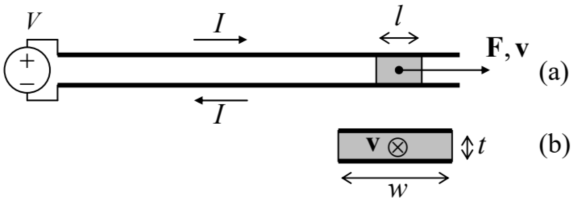
6.7. The electromagnetic railgun is a projectile launch system consisting of two long, parallel conducting rails and a sliding conducting projectile, shorting the current \(\ I\) fed into the system by a powerful source – see panel (a) in the figure on the right. Calculate the force exerted on the projectile, using two approaches:

(i) by a direct calculation, assuming that the cross-section of the system has the simple shape shown on panel (b) of the figure above, with \(\ t<<w\), \(\ l\), and

(ii) using the energy balance (for simplicity, neglecting the Ohmic resistances in the system), and compare the results.

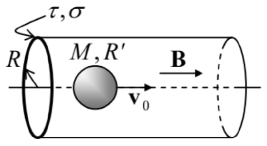
Screen Shot 2022-02-13 at 11.05.56 PM.png

6.8. A uniform, static magnetic field \(\ \mathbf{B}\) is applied along the axis of a long round pipe of a radius \(\ R\), and a very small thickness \(\ \tau\), made of a material with Ohmic conductivity \(\ \sigma\). A sphere of mass \(\ M\) and radius \(\ R^{\prime}<R\), made of a linear magnetic with permeability \(\ \mu >> \mu_{0}\), is launched, with an initial velocity \(\ \nu_{0}\), to fly ballistically along the pipe’s axis – see the figure on the right. Use the quasistatic approximation to calculate the distance the sphere would pass before it stops. Formulate the conditions of validity of your result.

Screen Shot 2022-02-13 at 11.11.22 PM.png

6.9. AC current of frequency \(\ \omega\) is being passed through a long uniform wire with a round cross-section of radius \(\ R\) comparable with the skin depth \(\ \delta_{\mathrm{s}}\). In the quasistatic approximation, find the current’s distribution across the cross-section, and analyze it in the limits \(\ R<<\delta_{\mathrm{s}}\) and \(\ \delta_{\mathrm{s}}<<R\). Calculate the effective ac resistance of the wire (per unit length) in these two limits.

6.10. A very long, round cylinder of radius R, made of a uniform conductor with an Ohmic conductivity \(\ \sigma\) and magnetic permeability \(\ \mu\), has been placed into a uniform ac magnetic field \(\ \mathbf{H}_{ext}(t)=\mathbf{H}_{0} \cos \omega t\), directed along its symmetry axis. Calculate the spatial distribution of the magnetic field’s amplitude, and in particular its value on the cylinder’s axis. Spell out the last result in the limits of relatively small and large \(\ R\).

6.11.^* Define and calculate an appropriate spatial-temporal Green’s function for Eq. (25), and then use this function to analyze the dynamics of propagation of the external magnetic field that is suddenly turned on at \(\ t = 0\) and then kept constant:

\(\ H(x<0, t)= \begin{cases}0, & \text { at } t<0 \\ H_{0}, & \text { at } t>0\end{cases}\)

into an Ohmic conductor occupying the semi-space \(\ x>0\) – see Fig. 2.

Hint: Try to use a function proportional to \(\ \exp \left\{-\left(x-x^{\prime}\right)^{2} / 2(\delta x)^{2}\right\}\), with a suitable time dependence of the parameter \(\ \delta x\), and a properly selected pre-exponential factor.

6.12. Solve the previous problem using the variable separation method, and compare the results.

6.13. A small, planar wire loop, carrying current \(\I\), is located far from a plane surface of a superconductor. Within the “coarse-grain” (ideal-diamagnetic) description of the Meissner-Ochsenfeld effect, calculate:

(i) the energy of the loop-superconductor interaction,

(ii) the force and torque acting on the loop, and

(iii) the distribution of supercurrents on the superconductor surface.

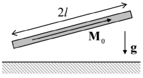
6.14. A straight, uniform magnet of length \(\ 2 l\), cross-section area \(\ A<<l^{2}\), and mass \(\ m\), with a permanent longitudinal magnetization \(\ M_{0}\), is placed over a horizontal surface of a superconductor – see the figure on the right. Within the ideal-diamagnet description of the Meissner-Ochsenfeld effect, find the stable equilibrium position of the magnet.

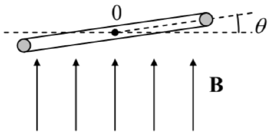
Screen Shot 2022-02-13 at 11.24.57 PM.png

6.15. A plane superconducting wire loop, of area \(\ A\) and inductance \(\ L\), may rotate, without friction, about a horizontal axis 0 (in the figure on the right, perpendicular to the plane of the drawing) passing through its center of mass. Initially, the loop was horizontal (with \(\ \theta=0\)), and carried supercurrent \(\ I_{0}\) in such direction that its magnetic dipole vector was directed down. Then a uniform magnetic field \(\ \mathbf{B}\), directed vertically up, was applied. Using the ideal-diamagnet description of the Meissner-Ochsenfeld effect, find all possible equilibrium positions of the loop, analyze their stability, and give a physical interpretation of the results.

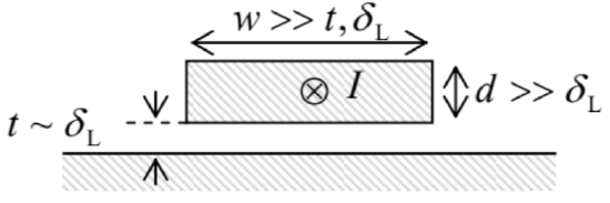
Screen Shot 2022-02-13 at 11.28.47 PM.png

6.16. Use the London equation to analyze the penetration of a uniform external magnetic field into a thin \(\ \left(t \sim \delta_{\mathrm{L}}\right)\), planar superconducting film, whose plane is parallel to the field.

6.17. Use the London equation to calculate the distribution of supercurrent density \(\ \mathbf{j}\) inside a long, straight superconducting wire, with a circular cross-section of radius \(\ R \sim \delta_{\mathrm{L}}\), carrying dc current \(\ I\).

6.18. Use the London equation to calculate the inductance (per unit length) of a long, uniform superconducting strip placed close to the surface of a similar superconductor – see the figure on the right, which shows the structure’s cross-section.

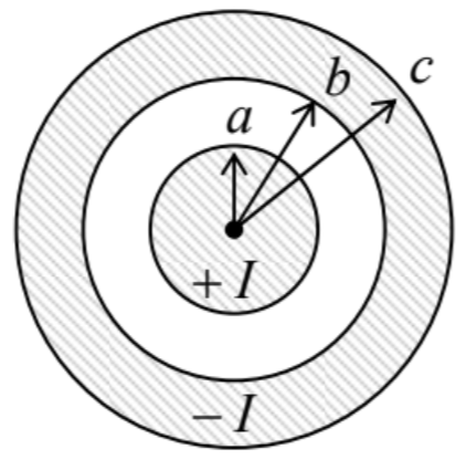
Screen Shot 2022-02-13 at 11.36.32 PM.png

6.19. Calculate the inductance (per unit length) of a superconducting cable with the round cross-section shown in the figure on the right, in the following limits:

(i) \(\ \delta_{\mathrm{L}}<<a, b, c-b\), and

(ii) \(\ a<<\delta_{\mathrm{L}}<<b, c-b\).

Screen Shot 2022-02-13 at 11.37.56 PM.png

6.20. Use the London equation to analyze the magnetic field shielding by a superconducting thin film of thickness \(\ t<<\delta_{\mathrm{L}}\), by calculating the penetration of the field induced by current \(\ I\) in a thin wire that runs parallel to a wide, plane, thin film, at distance \(\ d >> t\) from it, into the space behind the film.

6.21. Use the Ginzburg-Landau equations (54) and (63) to calculate the largest (“critical”) value of supercurrent in a uniform, long superconducting wire of a small cross-section \(\ A_{\mathrm{w}}<<\delta_{\mathrm{L}}^{2}\).

6.22. Use the discussion of a long, straight Abricosov vortex, in the limit \(\ \xi<<\delta_{\mathrm{L}}\), in Sec. 5 to prove Eqs. (71)-(72) for its energy per unit length, and the first critical field.

6.23.^* Use the Ginzburg-Landau equations (54) and (63) to prove the Josephson relation (76) for a small superconducting weak link, and express its critical current \(\ I_{\mathrm{c}}\) via the Ohmic resistance \(\ R_{\mathrm{n}}\) of the same weak link in its normal state.

6.24. Use Eqs. (76) and (79) to calculate the coupling energy of a Josephson junction and the full potential energy of the SQUID shown in Fig. 4c.

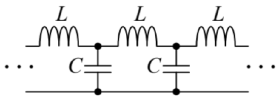
6.25. Analyze the possibility of wave propagation in a long, uniform chain of lumped inductances and capacitances – see the figure on the right.

Hint: Readers without prior experience with electromagnetic wave analysis may like to use a substantial analogy between this effect and mechanical waves in a 1D chain of elastically coupled particles.⁷⁵

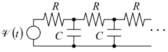
Screen Shot 2022-02-13 at 11.42.00 PM.png

6.26. A sinusoidal e.m.f. of amplitude \(\ V_{0}\) and frequency \(\ \omega\) is applied to an end of a long chain of similar, lumped resistors and capacitors, shown in the figure on the right. Calculate the law of decay of the ac voltage amplitude along the chain.

Screen Shot 2022-02-13 at 11.46.09 PM.png

6.27. As was discussed in Sec. 7, the displacement current concept allows one to generalize the Ampère law to time-dependent processes as

\[\ \oint_{C} \mathbf{H} \cdot d \mathbf{r}=I_{S}+\frac{\partial}{\partial t} \int_{S} D_{n} d^{2} r.\]

We also have seen that such generalization makes the integral \(\ \int \mathbf{H} \cdot d \mathbf{r}\) over an external contour, such as the one shown in Fig. 10, independent of the choice of the surface \(\ S\) limited by the contour. However, it may look like the situation is different for a contour drawn inside the capacitor – see the figure on the right. Indeed, if the contour’s size is much larger than the capacitor’s thickness, the magnetic field \(\ \mathbf{H}\), created by the linear current \(\ I\) on the contour’s line is virtually the same as that of a continuous wire, and hence the integral \(\ \int \mathbf{H} \cdot d \mathbf{r}\) along the contour apparently does not depend on its area, while the magnetic flux \(\ \int D_{n} d^{2} r\) does, so that the equation displayed above seems invalid. (The current \(\ I_{S}\) piercing this contour evidently equals zero.) Resolve the paradox, for simplicity considering an axially-symmetric system.

6.28. A straight, uniform, long wire with a circular cross-section of radius \(\ R\), is made of an Ohmic conductor with conductivity \(\ \sigma\), and carries dc current \(\ I\). Calculate the flux of the Poynting vector through its surface, and compare it with the Joule rate of energy dissipation.

Reference

⁷⁵ See, e.g., CM Sec. 6.3.