5.2: Rigid Body Rotation

In Equations 5.1.62-5.1.65 we have introduced the concept of time formally as a parameter to specify some simple types of motion which have a stationary character.

We examine now the usefulness of these results by considering the inertial motions of a rigid body fixed at one of its points, the so-called gyroscope.

We may sum up the relevant experimental facts as follows: there are objects of a sufficiently high symmetry (the spherical top) that indeed display a stationary, inertial rotation around any of their axes. In the general case (asymmetric top) such a stationary rotation is possible only around three principal directions marked out in the body triad.

The point of greatest interest for us, however, is the fact that there are also modes of motion that can be considered stationary in a weaker sense of the word.

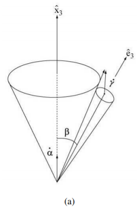
We mean the so-called precession. We shall consider here only the regular precession of the symmetric top, or gyroscope, that can be visualized in terms of the well known geometrical construction developed by Poinsot in 1853. The motion is produced by letting a circular cone fixed in the body triad \(\Sigma_{c}\) roll over a circular cone fixed in the space triad \(\Sigma_{s}\) (see Figure 5.2).

The noteworthy point is that the biaxial nature of spinors renders them well suited to provide an algebraic counterpart to this geometric picture.

In order to prove this point we have to make use of the theorem that angular velocities around different axes can be added according to the rules of vectorial addition. This theorem is a simple corollary of our formalism.

Let us consider the composition of infinitesimal rotations with \(\delta \phi=\omega \delta t<<1:\)

\[U_{2}\left(\hat{u}_{2}, \frac{\omega_{2} \delta t}{2}\right) U_{1}\left(\hat{u}_{1}, \frac{\omega_{1} \delta t}{2}\right) \simeq\left(1-\frac{\omega_{2} \delta t}{2} \hat{u}_{2} \cdot \vec{\sigma}\right)\left(1-\frac{\omega_{1} \delta t}{2} \hat{u}_{1} \cdot \vec{\sigma}\right)\label{1}\]

\[\simeq 1-\frac{\delta t}{2}\left(\omega_{2} \hat{u}_{2}+\omega_{1} \hat{u}_{1}\right) \cdot \vec{\sigma}\label{2}\]

We define the angular velocity vectors

\[\vec{\omega}=\omega \hat{u}\label{3}\]

and notice from Equation \ref{1} that

\[\vec{\omega}_{1}+\vec{\omega}_{2}=\vec{\omega}\label{4}\]

Consequently we obtain for the situation presented in Figure 5.2:

\[\vec{\omega}=\dot{\gamma} \hat{e}_{3}+\dot{\alpha} \hat{x}_{3}\label{5}\]

\[\omega^{2}=\dot{\alpha}^{2}+\dot{\gamma}^{2}+2 \dot{\alpha} \dot{\gamma} \cos \beta\label{6}\]

\[\beta=\hat{x}_{3} \cdot \hat{e}_{3}\label{7}\]

We can describe the precession in spinorial terms as follows. We describe the gyroscope configuration in terms of the unitary matrix 5.1.10 and operate on it from right and left with two unitary operators:

\[\begin{equation}
\begin{aligned}
V(t)=& U\left(\hat{x}_{3}, \frac{\dot{\alpha} t}{2}\right) V(0) U\left(\hat{e}_{3}, \frac{\dot{\gamma} t}{2}\right) \\
=&\left(\begin{array}{cc}
e^{-i \dot{\alpha} t / 2} & 0 \\
0 & e^{i \dot{\alpha} t / 2}
\end{array}\right)\left(\begin{array}{cc}
e^{-i \alpha(0) / 2} \cos (\beta / 2) e^{-i \gamma(0) / 2} & -e^{-i \alpha(0) / 2} \sin (\beta / 2) e^{i \gamma(0) / 2} \\
e^{i \alpha(0) / 2} \sin (\beta / 2) e^{-i \gamma(0) / 2} & e^{i \alpha(0) / 2} \cos (\beta / 2) e^{i \gamma(0) / 2}
\end{array}\right) \\
& \times\left(\begin{array}{cc}
e^{-i \dot{\gamma} t / 2} & 0 \\
0 & e^{i \dot{\gamma} t / 2}
\end{array}\right)
\end{aligned}
\end{equation}\label{8}\]

Thus

\[\alpha=\alpha(0)+\dot{\alpha} t, \quad \gamma=\gamma(0)+\dot{\gamma} t\label{9}\]

This relation displays graphically the biaxial character of the V matrix. Thus premultiplication corresponds to rotation in \(\Sigma_{s}\) and postmultiplication to that in \(\Sigma_{c}\).

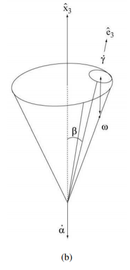
Note that the situations represented in Figure 5.2 (a) and (b) are called progressive and retrograde precessions respectively.

The rotational axis \(\vec{\omega}\) is instantaneously at rest in both frames. The vector components can be expressed as follows:

\[\begin{equation}
\begin{array}{c|c}
\Im \Sigma_{s} & \Im \Sigma_{c} \\
\hline \omega_{1}=\dot{\gamma} \sin \beta \cos \alpha & \omega_{1}=\dot{\alpha} \sin \beta \cos \gamma \\
\omega_{2}=\dot{\gamma} \sin \beta \sin \alpha & \omega_{2}=\dot{\alpha} \sin \beta \sin \gamma \\
\omega_{3}=\dot{\gamma} \cos \beta+\dot{\alpha} & \omega_{3}=\dot{\alpha} \cos \beta+\dot{\gamma}
\end{array}
\end{equation}\label{10}\]

These expressions can be derived formally from Equation \ref{8}. The left column of Equation \ref{10} follows from the application of the left-operator on a ket spinor and the right column of Equation \ref{10} from a right operation on a bra spinor.

Another way of arriving at these results is as follows: Expressions in the left column of Equation \ref{10} are evident from the vector addition rule given in \ref{4}. Expressions in the right column of Equation \ref{10} do not follow so easily from geometrical intuition. However, we can invoke the kinematic relativity between the two triads. A rotation of \(\Sigma_{c}\) with respect to \(\Sigma_{s}\) can be thought of also as the reverse rotation of \(\Sigma_{s}\) in \(\Sigma_{c}\). Thus \(V_{c}\) is equivalent to

\[V_{s}^{-1}=V_{s}^{\dagger}=V_{s}(-\alpha,-\beta,-\gamma)\label{11}\]

and we arrive from left to the right columns in Equation \ref{10} by the following substitution:

\[\alpha \rightarrow-\gamma\label{12}\]

\[\beta \rightarrow-\beta\label{13}\]

\[\gamma \rightarrow-\alpha\label{14}\]

\[t \rightarrow-t\label{15}\]

\[.........................................................................\label{16}\]

Up to this point the discussion has been only descriptive, kinematic. We have to turn to dynamics to answer the deeper questions as to the factors that determine the nature of the precession in any particular instance.

We invoke the kinematic relation Equation 5.1.62:

\[\exp \left(-i \frac{\omega t}{2} \hat{k} \cdot \vec{\sigma}\right)\left|\hat{k}, \frac{\gamma}{2}\right\rangle=\exp \left(-i \frac{\omega t}{2}\right)\left|\hat{k}, \frac{\gamma}{2}\right\rangle\label{17}\]

This expression offers a way of generalization to dynamics. If this relation indeed describes a stationary process, then the generators \(\frac{i}{2} \sigma_{j}\) of the unitary operator are constants of that motion. Later we shall pursue this idea to establish the concept of angular momentum and its quantizations. However, at this preliminary stage we are merely looking for an elementary illustration of the formalism, and we draw on the standard results of rigid body dynamics.

The dynamic law consists of three propositions. First, we have in \(\Sigma_{s}\)

\[\frac{d \vec{L}_{s}}{d t}=\vec{N}\label{18}\]

where N is the external torque.

In \(\Sigma_{c}\) we have a constitutive relation connecting angular velocity and angular momentum. We assume that the object triad is along the principal axes of inertia:

\[\begin{equation}
\begin{aligned}
L_{c 1} &=I_{1} \omega_{1} \\
L_{c 2} &=I_{2} \omega_{2} \\
L_{c 3} &=I_{3} \omega_{3}
\end{aligned}
\end{equation}\label{19}\]

Finally, the angular momentum components in \(\Sigma_{s} \text { and } \Sigma_{c}\) are connected by the relation

\[\frac{d \vec{L}_{s}}{d t}=\frac{d \vec{L}_{c}}{d t}+\vec{\omega} \times \vec{L}_{c}\label{20}\]

Equations \ref{18}–\ref{20} imply the Euler equations. Dynamically the precession may stem either from an external torque, or from the anisotropy of the moment of inertia (or both).

We shall assume \(\vec{N}=0 \text { and } I_{1}=I_{2} \neq I_{3}\). The Euler equations simplified accordingly yield for the precession as viewed in \(\Sigma_{c}\):

\[\begin{equation}
\begin{aligned}
\dot{\omega}_{c 1}+i \dot{\omega}_{c 2} &=-i\left(\omega_{c 1}+i \omega_{c 2}\right) \omega_{3} \delta \\
I_{3} \dot{\omega}_{3} &=0
\end{aligned}
\end{equation}\label{21}\]

with

\[\delta=1-\frac{I_{3}}{I_{1}}\label{22}\]

From Equation \ref{10}, right hand column, row (a) and (b), we obtain

\[\dot{\omega}_{1}+i \dot{\omega}_{2}=-i \dot{\gamma}\left(\omega_{1}+i \omega_{2}\right)\label{23}\]

and by comparison with \ref{21} we have

\[\dot{\gamma}=\omega_{3} \delta=\omega_{3}\left(1-\frac{I_{3}}{I_{1}}\right)\label{24}\]

We obtain from \ref{24}, \ref{22} and \ref{10} (the right hand column, row c):

\[I_{3} \omega_{3}=I_{1} \dot{\alpha} \cos \beta\label{25}\]

and

\[\frac{\dot{\gamma}}{\dot{\alpha} \cos \beta}=\frac{I_{1}}{I_{3}}-1\label{26}\]

Thus the nature of inertial precession is determined by the inertial anisotropy \ref{22}. In particular, let \(\cos \beta>0\), then

\[I_{1}>I_{3} \rightarrow \frac{\dot{\gamma}}{\dot{\alpha}}>0 \text { see Figure } 5.2 \text { -a }\label{27}\]

\[I_{1}<I_{3} \rightarrow \frac{\dot{\gamma}}{\dot{\alpha}}<0 \text { see Figure } 5.2-\mathrm{b}\label{28}\]

Finally, from Equation \ref{25} \(L_{c 3}=I_{3} \omega_{3}=I_{1} \dot{\alpha} \cos \beta\) and the total angular momentum squared is

\[L^{2}=I_{1}^{2} \dot{\alpha}^{2}\label{29}\]

Note that \(L_{c 3}=I_{1} \dot{\alpha} \cos \beta\) is the projection of the total angular momentum on to the figure axis. The precession \(\gamma \text { in } \Sigma_{c}\) comes about if \(I_{3} \neq I_{1}\). For further detail we refer to [KS65].

We note also that Euler’s theory has been translated into the modern language of Lie Groups by V. Arnold ([Arn66] pp 319-361). However in this work stationary motions are required to have fixed rotational axes.

Figure 5.2: Progressive (a) and Retrograde (b) Precession.