5.5: Review of SU(2) and preview of quantization


( \newcommand{\kernel}{\mathrm{null}\,}\)
Our introduction of the spinor concept at the beginning of Section 5.1 can be rationalized on the basis of the following guidelines. First, we require a certain economy and wish to avoid dealing with redundant parameters in specifying a rotating triad, just as we have previously solved the analogous problem for the rotation operator. Second, we wish to have an efficient formalism to represent the rotational problem.
We have seen that the matrices of SU(2) satisfy all these requirements, but we find ourselves saddled with a two-valuedness of the representation: |ξ⟩ and |ξ⟩ correspond to the same triad configuration. This is not a serious trouble, since our key relations 5.1.36 and 5.1.37 are quadratic in |ξ⟩. Thus the two-valuedness appears here only as a computational aid that disappears in the final result.
The situation is different if we look at the formulas 5.1.42–5.1.66 of the same section (Section 5.1). These equations are linear, they have a quantum mechanical character and we know that they are indeed applicable in the proper context. It is a pragmatic fact the two-valuedness is not just a necessary nuisance, but has physical meaning. But to understand this meaning is a challenge which we can meet only in carefully chosen steps.
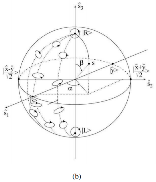
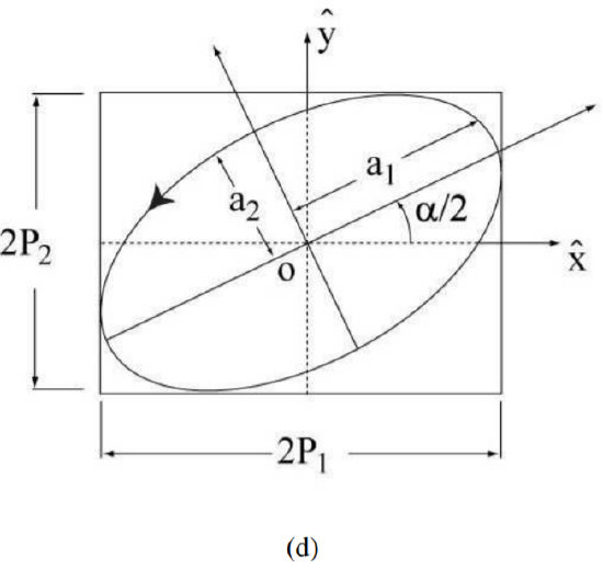
We wish to give a more physical interpretation to the triad, but avoid the impasse of the rigid body. First we associate the abstract Poincaré space with the physical system of the two-dimensional degenerate oscillator. The rotation in the Poincare´ space is associated with a phase shift between conjugate states, which is translated into a rotation of the Poincaré sphere, interpreted in turn as a change in orientation, or change of shape of the vibrational patterns in ordinary space.
It is only a mild exaggeration to say that our transition from the triad in Euclidean space to that in Poincare´ space is something like a “quantization,” in the sense as Schrödinger’ ¨ s wave equation associates a wave with a particle. (Planck’s h is to enter shortly!)
In this theory we have a good use for the conjugate spinors |ξ⟩ and |ˉξ⟩ representing opposite polarizations, but we must identify |ˉξ⟩=−|ξ⟩ with |ξ⟩.
The foregoing is still nothing but a perfectly well-defined kinematic model. The next step is different. As a “second quantization” we introduce Planck’s h to define single photons. A beam splitting represented by a projection operator can be expressed in probabilistic terms.
Formally all this is easy and we would at once have a great deal of the quantum mechanical formalism involving the theory of measurement.
Next, we could take the two-valuedness of the spinor seriously and obtain the formalism of isospin and of the neutrino, say as in Section 17, Fermion States, in [Kae65].
Finally, instead of doubly degenerate vibrations, we could consider the triply degenerate vibrator and handle it by SU(3) [Lip02] . We shall not consider these generalizations at this point, however. Before further expanding the formalism we should hope to understand better what we already have.
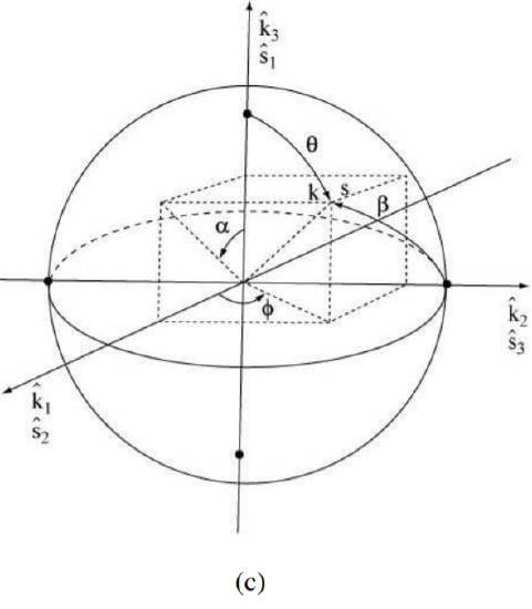
First, a formal remark. Our results thus far developed are uniquely determined by the spinor formalism of Section 5.1 and by the program of considering the Poincaré sphere as the basic configuration space to be described by conventional spherical coordinates α,β or ϕ,θ.
It is noteworthy that this modest conceptual equipment carries us so far. We have obtained spinors, density matrices and have discussed at least fleetingly coherence, incoherence, quantum theory of measurement and transformation theory.
What we do not get out of the theory is a specific interpretation of the underlying vibrational process since the formalism is thus far entirely independent of it. This fact gives us some understanding of the scope and limit of quantum mechanics. We can apply the formalism to phenomena we understand very little. However, since the same §U(2) formalism applies to polarized light, spin, isospin, strangeness and other phenomena, we learn little about their distinctive aspects.
In order to overcome this limitation we need a deeper understanding of what a quantized angular momentum is in the framework of a dynamical problem.
The next chapter is devoted to a phenomenological discussion of the concepts of particle and wave. We shall attempt to obtain sufficient hints for developing a dynamic theory in the form of a phase space geometry in Chapter VI.