8.2: Branches

We have discussed two examples of multi-valued complex operations: non-integer powers and the complex logarithm. However, we usually prefer to deal with functions rather than multi-valued operations. One major motivating factor is that the concept of the complex derivative was formulated in terms of functions, not multi-valued operations.

There is a standard procedure to convert multi-valued operations into functions. First, we define one or more curve(s) in the complex plane, called branch cuts (the reason for this name will be explained later). Next, we modify the domain (i.e., the set of permissible inputs) by excluding all values of \(z\) lying on a branch cut. Then the outputs of the multi-valued operation can be grouped into discrete branches, with each branch behaving just like a function.

The above procedure can be understood through the example of the square root.

Branches of the complex square root

As we saw in Section 8.1, the complex square root, \(z^{1/2}\), has two possible values. We can define the two branches as follows:

1. Define a branch cut along the negative real axis, so that the domain excludes all values of \(z\) along the branch cut. In in other words, we will only consider complex numbers whose polar representation can be written as \[z = r e^{i\theta}, \quad \theta \in (-\pi, \pi).\] (For those unfamiliar with this notation, \(\theta \in (-\pi, \pi)\) refers to the interval \(-\pi < \theta < \pi\). The parentheses indicate that the boundary values of \(-\pi\) and \(\pi\) are excluded. By contrast, we would write \(\theta \in [-\pi, \pi]\) to refer to the interval \(-\pi \le \theta \le \pi\), with the square brackets indicating that the boundary values are included.)

2. One branch is associated with the \(+1\) root. On this branch, for \(z = re^{i\theta}\), the value is \[f_+(z) = r^{1/2} \, e^{i\theta/2}, \quad \theta \in (-\pi, \pi).\]

3. The other branch is associated with the root of unity \(-1\). On this branch, the value is \[f_-(z) = -r^{1/2} \, e^{i\theta/2}, \quad \theta \in (-\pi, \pi).\]

In the following plot, you can observe how varying \(z\) affects the positions of \(f_+(z)\) and \(f_-(z)\) in the complex plane:

Figure \(\PageIndex{1}\)

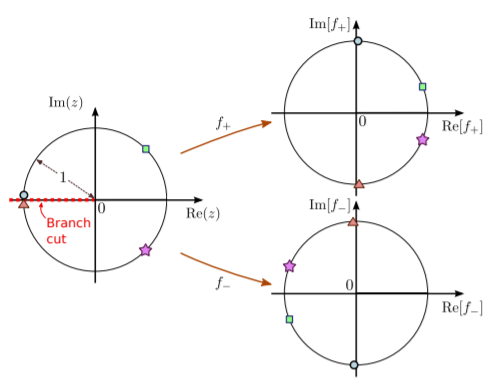
The red dashed line in the left plot indicates the branch cut. Our definitions of \(f_+(z)\) and \(f_-(z)\) implicitly depend on the choice to place the branch cut on the negative real axis, which led to the representation of the argument of \(z\) as \(\theta \in (-\pi,\pi)\).

In the above figure, note that \(f_+(z)\) always lies in the right half of the complex plane, whereas \(f_-(z)\) lies in the left half of the complex plane. Both \(f_+\) and \(f_-\) are well-defined functions with unambiguous outputs, albeit with domains that do not cover the entire complex plane. Moreover, they are analytic over their entire domain (i.e., all of the complex plane except the branch cut); this can be proven using the Cauchy-Riemann equations, and is left as an exercise.

The end-point of the branch cut is called a branch point. For \(z = 0\), both branches give the same result: \(f_+(0) = f_-(0) = 0\). We will have more to say about branch points in Section 8.2.

Different branch cuts for the complex square root

In the above example, you may be wondering why the branch cut has to lie along the negative real axis. In fact, this choice is not unique. For instance, we could place the branch cut along the positive real axis. This corresponds to specifying the input \(z\) using a different interval for \(\theta\): \[z = re^{i\theta}, \quad \theta \in (0, 2\pi).\] Next, we use the same formulas as before to define the branches of the complex square root: \[f_\pm(z) = \pm r^{1/2} \, e^{i\theta/2}.\] But because the domain of \(\theta\) has been changed to \((0, 2\pi)\), the set of inputs \(z\) now excludes the positive real axis. With this new choice of branch cut, the branches are shown in the following figure.

Figure \(\PageIndex{2}\)

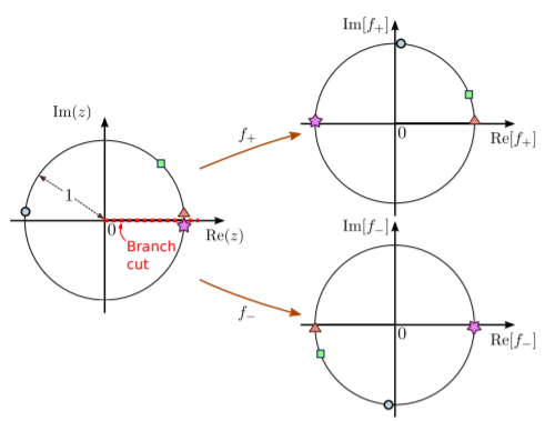
These two branch functions are different from what we had before. Now, \(f_+(z)\) is always in the upper half of the complex plane, and \(f_-(z)\) in the lower half of the complex plane. However, both branches still have the same value at the branch point: \(f_+(0) = f_-(0) = 0\).

The branch cut serves as a boundary where two branches are “glued” together. You can think of “crossing” a branch cut as having the effect of moving continuously from one branch to another. In the above figure, consider the case where \(z\) is just above the branch cut. Then \(f_+(z)\) lies just above the positive real axis, and \(f_-(z)\) lies just below the negative real axis. Next, consider \(z\) lying just below the branch cut. This is equivalent to a small downwards displacement of \(z\), “crossing” the branch cut. For this case, \(f_-(z)\) now lies just below the positive real axis, near where \(f_+(z)\) was previously. Moreover, \(f_+(z)\) now lies just above the negative real axis, near where \(f_-(z)\) was previously. Crossing the branch cut thus swaps the values of the positive and negative branches.

The three-dimensional plot below provides another way to visualize the role of the branch cut. Here,the horizontal axes correspond to \(\mathrm{Re}(z)\) and \(\mathrm{Im}(z)\). The vertical axis shows the arguments for the two values of the complex square root, with \(\mathrm{arg}\big[f_+(z)\big]\) plotted in orange and \(\mathrm{arg}\big[f_-(z)\big]\) plotted in blue. If we vary the choice of the branch cut, that simply affects which values of the multi-valued operation are assigned to the \(+\) (orange) branch, and which values are assigned to the \(-\) (blue) branch. Hence, the choice of branch cut is just a choice about how to divide up the branches of a multi-valued operation.

Figure \(\PageIndex{3}\)

Branch points

The tip of each branch cut is called a branch point. A branch point is a point where the multi-valued operation gives an unambiguous answer, with different branches giving the same output. Whereas the choice of branch cuts is non-unique, the positions of the branch points of a multi-valued operation are uniquely determined.

For the purposes of this course, you mostly only need to remember the branch points for two common cases:

• The \(z^p\) operation (for non-integer \(p\)) has branch points at \(z = 0\) and \(z = \infty\). For rational powers \(p = P/Q\), where \(P\) and \(Q\) have no common divisor, there are \(Q\) branches, one for each root of unity. At each branch point, all \(Q\) branches meet.

• The complex logarithm has branch points at \(z = 0\) and \(z = \infty\). There is an infinite series of branches, separated from each other by multiples of \(2 \pi i\). At each branch point, all the branches meet.

We can easily see that \(z^p\) must have a branch point at \(z = 0\): its only possible value at the origin is \(0\), regardless of which root of unity we choose. To understand the other branch points listed above, a clearer understanding of the concept of “infinity” for complex numbers is required, so we will discuss that now.