10.1: Fourier Series

We begin by discussing the Fourier series, which is used to analyze functions that are periodic in their inputs. A periodic function \(f(x)\) is a function of a real variable \(x\) that repeats itself every time \(x\) changes by \(a\), as shown in the figure below:

Figure \(\PageIndex{1}\)

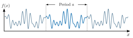
The constant \(a\) is called the period. Mathematically, we write the periodicity condition as \[f(x+a) = f(x), \quad\forall\;\, x\in \mathbb{R}.\] The value of \(f(x)\) can be real or complex, but \(x\) should be real. You can think of \(x\) as representing a spatial coordinate. (The following discussion also applies to functions of time, though with minor differences in convention that are discussed in Section 10.3.) We can also think of the periodic function as being defined over a finite segment \(-a/2 \le x < a/2\), with periodic boundary conditions \(f(-a/2) = f(a/2)\). In spatial terms, this is like wrapping the segment into a loop:

Figure \(\PageIndex{2}\)

Let’s consider what it means to specify a periodic function \(f(x)\). One way to specify the function is to give an explicit mathematical formula for it. Another approach might be to specify the function values in \(-a/2 \le x < a/2\). Since there’s an uncountably infinite number of points in this domain, we can generally only achieve an approximate specification of \(f\) this way, by giving the values of \(f\) at a large but finite set \(x\) points.

There is another interesting approach to specifying \(f\). We can express it as a linear combination of simpler periodic functions, consisting of sines and cosines: \[f(x) = \sum_{n=1}^\infty \alpha_n \sin\left(\frac{2\pi n x}{a}\right) + \sum_{m=0}^\infty \beta_m \cos\left(\frac{2 \pi m x}{a}\right).\] This is called a Fourier series. Given the set of numbers \(\{\alpha_n, \beta_m\}\), which are called the Fourier coefficients, \(f(x)\) can be calculated for any \(x\). Note that the Fourier coefficients are real if \(f(x)\) is a real function, or complex if \(f(x)\) is complex.

The justification for the Fourier series formula is that the sine and cosine functions in the series are, themselves, periodic with period \(a\): \[\begin{align} \sin\left(\frac{2\pi n (x+a)}{a}\right) = \sin\left(\frac{2\pi n x}{a} + 2\pi n\right) &= \sin\left(\frac{2\pi n x}{a}\right) \\ \cos\left(\frac{2\pi m (x+a)}{a}\right) = \cos\left(\frac{2\pi m x}{a} + 2\pi m\right) &= \cos\left(\frac{2\pi m x}{a}\right).\end{align}\] Hence, any linear combination of them automatically satisfies the periodicity condition for \(f\). (Note that in the Fourier series formula, the \(n\) index does not include 0. Since the sine term with \(n = 0\) vanishes for all \(x\), it’s redundant.)

Square-integrable functions

The Fourier series is a nice concept, but can arbitrary periodic functions always be expressed as a Fourier series? This question turns out to be surprisingly intricate, and its resolution preoccupied mathematicians for much of the 19th century. The full discussion is beyond the scope of this course.

Luckily, it turns out that a certain class of periodic functions, which are commonly encountered in physical contexts, are guaranteed to always be expressible as Fourier series. These are square-integrable functions, for which \[\int_{-a/2}^{a/2} dx\; \big|\,f(x)\,\big|^2\;\;\text{exists and is finite}.\] Unless otherwise stated, we will always assume that the functions we’re dealing with are square-integrable.

Complex Fourier series and inverse relations

Using Euler’s formula, we can re-write the Fourier series as follows: \[f(x) = \sum_{n=-\infty}^\infty e^{2\pi i n x/a}\, f_n.\] Instead of separate sums over sines and cosines, we have a single sum over complex exponentials, which is neater. The sum includes negative integers \(n\), and involves a new set of Fourier coefficients, \(f_n\), which are complex numbers. (As an exercise, try working out how the old coefficients \(\{\alpha_n, \beta_n\}\) are related to the new coefficients \(\{f_n\}\).)

If the Fourier coefficients \(\{f_n\}\) are known, then \(f(x)\) can be calculated using the above formula. The converse is also true: given \(f(x)\), we can determine the Fourier coefficients. To see how, observe that \[\int_{-a/2}^{a/2} dx \; e^{-2\pi i m x/a}\, e^{2\pi i n x/a} = a\, \delta_{mn}\quad \mathrm{for}\;m, n \in \mathbb{Z},\] where \(\delta_{mn}\) is the Kronecker delta, defined as: \[\delta_{mn} = \left\{\begin{array}{ll}1, & \textrm{if}\; m = n\\ 0, & \mathrm{if}\;m\ne n.\end{array}\right.\] Due to this property, the set of functions \(\exp(2\pi i n x / a)\), with integer values of \(n\), are said to be orthogonal functions. (We won’t go into the details now, but the term “orthogonality” is used here with the same meaning as in vector algebra, where a set of vectors \(\vec{v}_1, \vec{v}_2, \dots\) is said to be “orthogonal” if \(\vec{v}_m \cdot \vec{v}_n = 0\) for \(m\ne n\).) Hence, \[\begin{align} \int_{-a/2}^{\,a/2} dx\; e^{-2\pi i m x/a} \;f(x) &= \, \int_{-a/2}^{\,a/2} dx\; e^{-2\pi i m x/a} \left[\sum_{n=-\infty}^\infty e^{2\pi i n x/a}\, f_n\right] \\ &= \sum_{n=-\infty}^\infty \, \int_{-a/2}^{\,a/2} dx\; e^{-2\pi i m x/a} \, e^{2\pi i n x/a} \;f_n \\ &= \sum_{n=-\infty}^\infty \, a\, \delta_{mn} \, f_n \\ &= a \,f_m.\end{align}\] The procedure of multiplying by \(\exp(-2\pi i m x/a)\) and integrating over \(x\) acts like a sieve, filtering out all other Fourier components of \(f(x)\) and keeping only the one with the matching index \(m\). Thus, we arrive at a pair of relations expressing \(f(x)\) in terms of its Fourier components, and vice versa:

Theorem \(\PageIndex{1}\)

\[\left\{\;\;\begin{array}{rl}f(x) &= \displaystyle \, \sum_{n=-\infty}^\infty e^{i k_n x}\, f_n \\ f_n &= \displaystyle\,\frac{1}{a} \int_{-a/2}^{\,a/2} dx\; e^{-i k_n x}\, f(x)\end{array}\;\;\right. \quad\quad\mathrm{where}\;\; k_n \equiv \frac{2\pi n}{a} \label{fseries-relations}\]

The real numbers \(k_n\) are called wave-numbers. They form a discrete set, with one for each Fourier component. In physics jargon, we say that the wave-numbers are “quantized” to integer multiples of \(\Delta k \equiv 2\pi/a.\)

Example: Fourier series of a square wave

To get a feel for how the Fourier series behaves, let’s look at a square wave: a function that takes only two values \(+1\) or \(-1\), jumping between the two values at periodic intervals. Within one period, the function is \[f(x) = \left\{\begin{array}{ll}-1, & -a/2 \le x < 0 \\ +1, & \quad\;\;\; 0 \le x < a/2.\end{array}\right.\] Plugging this into the Fourier relation, and doing the straightforward integrals, gives the Fourier coefficients \[\begin{align} f_n &= -i \, \frac{\left[\sin\left(n \pi/2\right)\right]^2}{n\pi/2 } \\ &= \left\{\begin{array}{cl} -2i/n\pi ,& n \; \mathrm{odd} \\ 0,& n \; \mathrm{even}. \end{array} \right.\end{align}\] As can be seen, the Fourier coefficients become small for large \(n\). We can write the Fourier series as \[f(x) \; \leftrightarrow \; \sum_{n=1,3,5,\dots} \frac{4\sin(2\pi n x / a)}{n \pi}.\] If this infinite series is truncated to a finite number of terms, we get an approximation to \(f(x)\). As shown in the figure below, the approximation becomes better and better as more terms are included.

Figure \(\PageIndex{2}\)

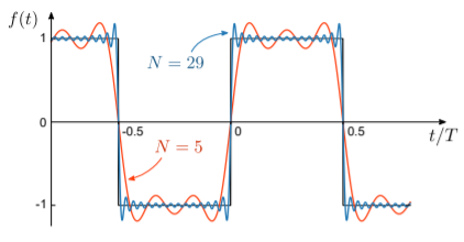
One amusing consequence of the above result is that we can use it to derive a series expansion for \(\pi\). If we set \(x = a/4\), \[f(a/4) = 1 = \frac{4}{\pi} \left[\sin(\pi/2) + \frac{1}{3}\sin(3\pi/2) + \frac{1}{5}\sin(5\pi/2) + \cdots\right],\] and hence \[\pi = 4 \left(1 - \frac{1}{3} + \frac{1}{5} - \frac{1}{7} + \cdots\right).\]