10.2: Fourier Transforms

The Fourier series applies to periodic functions defined over the interval $-a/2 \le x < a/2$. But the concept can be generalized to functions defined over the entire real line, $x \in \mathbb{R}$, if we take the limit $a \rightarrow \infty$ carefully.

Suppose we have a function $f$ defined over the entire real line, $x \in \mathbb{R}$, such that $f(x) \rightarrow 0$ for $x \rightarrow \pm\infty$. Imagine there is a family of periodic functions $\big\{f_a(x) \,\big|\, a \in\mathbb{R}^+\big\}$, such that $f_a(x)$ has periodicity $a$, and approaches $f(x)$ in the limit $a\rightarrow \infty$. This is illustrated in the figure below:

Figure $\PageIndex{1}$

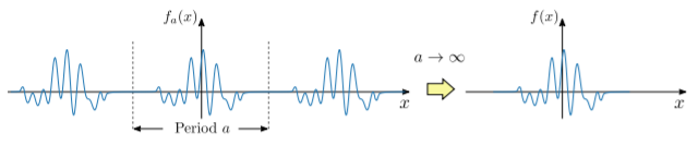
In mathematical terms, $$f(x) = \lim_{a \rightarrow \infty} f_a(x), \;\;\;\text{where}\;\; f_a(x+a) = f_a(x).$$ Since $f_a$ is periodic, it can be expanded as a Fourier series: $$f_a(x) = \sum_{n=-\infty}^\infty e^{i k_n x}\, f_{an}, \quad\mathrm{where}\;\; k_n = n\Delta k, \;\; \Delta k = \frac{2\pi}{a}.$$ Here, $f_{an}$ denotes the $n$-th complex Fourier coefficient of the function $f_a(x)$. Note that each Fourier coefficient depends implicitly on the periodicity $a$.

As $a \rightarrow \infty$, the wave-number quantum $\Delta k$ goes to zero, and the set of discrete $k_n$ turns into a continuum. During this process, each individual Fourier coefficient $f_{an}$ goes to zero, because there are more and more Fourier components in the vicinity of each $k$ value, and each Fourier component contributes less. This implies that we can replace the discrete sum with an integral. To accomplish this, we first multiply the summand by a factor of $(\Delta k/2\pi) / (\Delta k/2\pi) = 1$: $$f(x) = \lim_{a\rightarrow \infty} \left[\;\,\sum_{n=-\infty}^\infty \frac{\Delta k}{2\pi} \, e^{i k_n x}\, \left(\frac{2\pi \,f_{an}}{\Delta k} \right)\;\,\right].$$ (In case you’re wondering, the choice of $2\pi$ factors is essentially arbitrary; we are following the usual convention.) Moreover, we define $$F(k) \equiv \lim_{a \rightarrow \infty} \left[\frac{2\pi\, f_{an}}{\Delta k}\right]_{k = k_n}.$$ In the $a \rightarrow \infty$ limit, the $f_{an}$ in the numerator and the $\Delta k$ in the denominator both go zero, but if their ratio remains finite, we can turn the Fourier sum into the following integral: $$f(x) = \int_{-\infty}^{\infty} \frac{dk}{2\pi} \, e^{i k x}\, F(k). \label{Fk}$$

The Fourier relations

The function $F(k)$ in Eq. $\eqref{Fk}$ is called the Fourier transform of $f(x)$. Just as we have expressed $f(x)$ in terms of $F(k)$, we can also express $F(k)$ in terms of $f(x)$. To do this, we apply the $a \rightarrow \infty$ limit to the inverse relation for the Fourier series in Eq. (10.1.13): $$\begin{align} F(k_n) &= \lim_{a\rightarrow \infty} \frac{2 \pi\, f_{an}}{\Delta k} \\ &= \lim_{a\rightarrow \infty} \frac{2 \pi}{2\pi/a}\, \left(\frac{1}{a} \int_{-a/2}^{a/2} dx\; e^{-i k_n x}\right) \\ &= \int_{-\infty}^\infty dx\; e^{-i kx}\, f(x).\end{align}$$ Hence, we arrive at a pair of equations called the Fourier relations:

Definition: Fourier relations

$$\begin{align}\left\{\;\;\begin{aligned}F(k) &= \;\int_{-\infty}^\infty dx\; e^{-ikx}\, f(x) &&\text{(Fourier transform)}\\ f(x) &= \int_{-\infty}^\infty \frac{dk}{2\pi}\; e^{ikx}\, F(k)&&\text{(Inverse Fourier transform).}\end{aligned}\;\;\right. \end{align} \label{fourier-relations}$$

The first equation is the Fourier transform, and the second equation is called the inverse Fourier transform.

There are notable differences between the two formulas. First, there is a factor of $1/2\pi$ appears next to $dk$, but no such factor for $dx$; this is a matter of convention, tied to our earlier definition of $F(k)$. Second, the integral over $x$ contains a factor of $e^{-ikx}$ but the integral over $k$ contains a factor of $e^{ikx}$. One way to remember which equation has the positive sign in the exponent is to interpret the inverse Fourier transform equation (which has the form of an integral over $k$) as the continuum limit of a sum over complex waves. In this sum, $F(k)$ plays the role of the series coefficients, and by convention the complex waves have the form $\exp(ikx)$ (see Section 6.3).

As noted in Section 10.1, all the functions we deal with are assumed to be square integrable. This includes the $f_a$ functions used to define the Fourier transform. In the $a \rightarrow \infty$ limit, this implies that we are dealing with functions such that $$\int_{-\infty}^{\infty} dx\; \big|\,f(x)\,\big|^2\;\;\text{exists and is finite}.$$

A simple example

Consider the function $$f(x) = \left\{\begin{array}{cl}e^{-\eta x}, & x \ge 0 \\ 0, & x < 0,\end{array}\right. \qquad \eta \in \mathbb{R}^+.$$ For $x < 0$, this is an exponentially-decaying function, and for $x < 0$ it is identically zero. The real parameter $\eta$ is called the decay constant; for $\eta > 0$, the function $f(x)$ vanishes as $x \rightarrow +\infty$ and can thus be shown to be square-integrable. Larger values of $\eta$ correspond to faster exponential decay.

The Fourier transform can be found by directly calculating the Fourier integral: $$F(k) \;=\; \;\int_{0}^\infty dx\; e^{-i kx}\, e^{-\kappa x} \;=\; \frac{-i}{k - i \eta}.$$ It is useful to plot the squared magnitude of the Fourier transform, $|F(k)|^2$, against $k$. This is called the Fourier spectrum of $f(x)$. In this case, $$\big|\,F(k)\,\big|^2 = \frac{1}{k^2 + \eta^2}.$$

Figure $\PageIndex{2}$

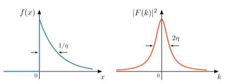
The Fourier spectrum is shown in the right subplot above. It consists of a peak centered at $k = 0$, forming a curve called a Lorentzian. The width of the Lorentzian is dependent on the original function’s decay constant $\eta$. For small $\eta$, i.e. weakly-decaying $f(x)$, the peak is narrow; for large $\eta$, i.e. rapidly-decaying $f(x)$, the peak is broad.

We can quantify the width of the Lorentzian by defining the full-width at half-maximum (FWHM)—the width of the curve at half the value of its maximum. In this case, the maximum of the Lorentzian curve occurs at $k=0$ and has the value of $1/\eta^2$. The half-maximum, $1/2\eta^2$, occurs when $\delta k = \pm \eta$. Hence, the original function’s decay constant, $\eta$, is directly proportional to the FWHM of the Fourier spectrum, which is $2\eta$.

To wrap up this example, let’s evaluate the inverse Fourier transform: $$f(x) \; = \; -i\int_{-\infty}^\infty \frac{dk}{2\pi} \; \frac{e^{i kx}}{k-i\eta}.$$ This can be solved by contour integration. The analytic continuation of the integrand has a simple pole at $k = i\eta$. For $x < 0$, the numerator $\exp(ikx)$ vanishes far from the origin in the lower half-plane, so we close the contour below. This encloses no pole, so the integral is zero. For $x > 0$, the numerator vanishes far from the origin in the upper half-plane, so we close the contour above, with a counter-clockwise arc, and the residue theorem gives $$f(x) = \left(\frac{-i}{2\pi}\right) \, \left(2\pi i\right) \, \mathrm{Res}\left[ \frac{e^{ikx}}{k-i\eta}\right]_{k=i\eta} = e^{-\eta x} \qquad(x > 0),$$ as expected.