10.6: Common Fourier Transforms

To accumulate more intuition about Fourier transforms, let us examine the Fourier transforms of some interesting functions. We will just state the results; the calculations are left as exercises.

Damped waves

We saw in Section 10.2 that an exponentially decay function with decay constant $\eta \in \mathbb{R}^+$ has the following Fourier transform:

$$f(x) = \left\{\begin{array}{cl}e^{-\eta x}, & x \ge 0 \\ 0, & x < 0,\end{array}\right. \;\; \overset{\mathrm{FT}}{\longrightarrow} \;\; F(k) = \frac{-i}{k-i\eta}.$$ Observe that $F(k)$ is given by a simple algebraic formula. If we “extend” the domain of $k$ to complex values, $F(k)$ corresponds to an analytic function with a simple pole in the upper half of the complex plane, at $k = i\eta$.

Next, consider a decaying wave with wave-number $q \in \mathbb{R}$ and decay constant $\eta \in \mathbb{R}^+$. The Fourier transform is a function with a simple pole at $q + i \eta$:

$$f(x) = \left\{\begin{array}{cl}e^{i (q + i\eta) x}, & x \ge 0 \\ 0, & x < 0.\end{array}\right. \;\; \overset{\mathrm{FT}}{\longrightarrow} \;\; F(k) = \frac{-i}{k-(q + i\eta)}.$$

On the other hand, consider a wave that grows exponentially with $x$ for $x < 0$, and is zero for $x > 0$. The Fourier transform is a function with a simple pole in the lower half-plane:

$$f(x) = \left\{\begin{array}{cl}0, & x \ge 0 \\ e^{i (q - i\eta) x}, & x < 0.\end{array}\right. \;\; \overset{\mathrm{FT}}{\longrightarrow} \;\; F(k) = \frac{i}{k-(q - i\eta)}.$$ From these examples, we see that oscillations and amplification/decay in $f(x)$ are related to the existence of poles in the algebraic expression for $F(k)$. The real part of the pole position gives the wave-number of the oscillation, and the distance from the pole to the real axis gives the amplification or decay constant. A decaying signal produces a pole in the upper half-plane, while a signal that is increasing exponentially with $x$ produces a pole in the lower half-plane. In both cases, if we plot the Fourier spectrum of $|F(k)|^2$ versus real $k$, the result is a Lorentzian peak centered at $k = q$, with width $2\eta$.

Gaussian wave-packets

Consider a function with a decay envelope given by a Gaussian function:

$$f(x) = e^{iq x} \, e^{-\gamma x^2}, \;\;\;\mathrm{where}\; q \in \mathbb{C},\; \gamma \in \mathbb{R}.$$ This is called a Gaussian wave-packet. The width of the envelope is usually characterized by the Gaussian function’s standard deviation, which is where the curve reaches $e^{-1/2}$ times its peak value. In this case, the standard deviation is $\Delta x = 1/\sqrt{2\gamma}$.

We will show that $f(x)$ has the following Fourier transform:

$$F(k) = \sqrt{\frac{\pi}{\gamma}} \, e^{-\frac{(k-q)^2}{4\gamma}}.$$

To derive this result, we perform the Fourier integral as follows:

$$\begin{align} F(k) &= \int_{-\infty}^\infty dx \, e^{-ikx}\, f(x) \\ &= \int_{-\infty}^\infty dx \, \exp\left\{-i(k-q)x -\gamma x^2\right\}.\end{align}$$ In the integrand, the expression inside the exponential is quadratic in $x$. We complete the square: $$\begin{align} F(k) &= \int_{-\infty}^\infty dx \, \exp\left\{-\gamma\left(x + \frac{i(k-q)}{2\gamma}\right)^2 + \gamma\left(\frac{i(k-q)}{2\gamma}\right)^2\right\} \\ &= \exp\left\{ - \frac{(k-q)^2}{4\gamma}\right\}\; \int_{-\infty}^\infty dx \, \exp\left\{-\gamma\left(x + \frac{i(k-q)}{2\gamma}\right)^2\right\}.\end{align}$$ The remaining integral is the Gaussian integral with a constant imaginary shift in $x$. By shifting the integration variable, one can show that this is equal the standard Gaussian integral, $\sqrt{\pi/\gamma}$; the details are left as an exercise. We thus arrive at the result stated above.

The Fourier spectrum, $|F(k)|^2$, is a Gaussian function with standard deviation

$$\Delta k = \frac{1}{\sqrt{2(1/2\gamma)}} = \sqrt{\gamma}.$$

Figure $\PageIndex{1}$

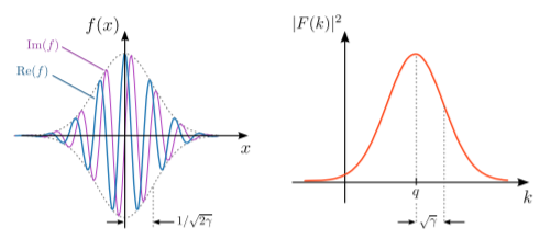
Once again, the Fourier spectrum is peaked at a value of $k$ corresponding to the wave-number of the underlying sinusoidal wave in $f(x)$, and a stronger (weaker) decay in $f(x)$ leads to a broader (narrower) Fourier spectrum. These features can be observed in the plot above.