9.1: Mid-Point Rule

The simplest numerical integration method is called the mid-point rule. Consider a definite 1D integral

\[\mathcal{I} = \int_a^b f(x) \, dx.\]

Let us divide the range \(a \le x \le b\) into a set of \(N\) segments of equal width, as shown in Fig. \(\PageIndex{1}\) for the case of \(N=5\). The mid-points of these segments are a set of \(N\) discrete points \(\{x_0, \dots x_{N-1}\}\), where

\[x_n = a + \left(n + \frac{1}{2}\right)\,\Delta x ,\quad \Delta x \equiv \frac{b-a}{N}.\]

We then estimate the integral as

\[\mathcal{I}^{\mathrm{(mp)}} = \Delta x \; \sum_{n=0}^{N-1} f(x_n) \;\;\;\overset{N\rightarrow\infty}{\longrightarrow} \;\;\; \mathcal{I}.\]

Figure \(\PageIndex{1}\): Computing a definite integral using the mid-point rule.

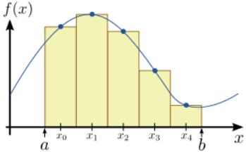
The principle behind this formula is very simple to understand. As shown in Fig. \(\PageIndex{1}\), \(I_{N}\) represents the area enclosed by a sequence of rectangles, where the height of each rectangle is equal to the value of \(f(x)\) at its mid-point. As \(N \rightarrow \infty\), the spacing between rectangles goes to zero; hence, the total area enclosed by the rectangles becomes equal to the area under the curve of \(f(x)\).

9.1.1 Numerical Error for the Mid-Point Rule

Let us estimate the numerical error resulting from this approximation. To do this, consider one of the individual segments, which is centered at \(x_n\) with length \(\Delta x = (b-a)/N\). Let us define the integral over this segment as

\[\Delta \mathcal{I}_n \equiv \int_{x_n - \Delta x/2}^{x_n + \Delta x/2} f(x) dx.\]

Now, consider the Taylor expansion of \(f(x)\) in the vicinity of \(x_{n}\):

\[f(x) = f(x_n) + f'(x_n) (x-x_n) + \frac{f''(x_n)}{2} (x-x_n)^2 + \frac{f'''(x_n)}{6} (x-x_n)^3 + \cdots \]

If we integrate both sides of this equation over the segment, the result is

\[\begin{align}\Delta\mathcal{I}_n \; = \; f(x_n) \Delta x \;\,&+\; f'(x_n) \int_{x_n - \Delta x/2}^{x_n + \Delta x/2} (x-x_n) dx\\ &+\; \frac{f''(x_n)}{2} \int_{x_n - \Delta x/2}^{x_n + \Delta x/2} (x-x_n)^2 dx\\ &+\; \cdots\end{align}\]

On the right hand side, every other term involves an integrand which is odd around \(x_{n}\). Such terms integrate to zero. From the remaining terms, we find the following series for the integral of \(f(x)\) over the segment:

\[\Delta\mathcal{I}_n \; = \; f(x_n) \Delta x \;+\; \frac{f''(x_n) \Delta x^3}{24} + O(\Delta x^5).\]

By comparison, the estimation provided by the mid-point rule is simply

\[\Delta \mathcal{I}^{\mathrm{mp}}_n = f(x_n) \Delta x\]

This is simply the first term in the exact series. The remaining terms constitute the numerical error in the mid-point rule integration, over this segment. We denote this error as

\[\mathcal{E}_n = \left|\Delta \mathcal{I}_n - \Delta \mathcal{I}_n^{\mathrm{mp}}\right| \;\sim\; \frac{|f''(x_n)|}{24} \Delta x^3 \;\sim\; O\left(\frac{1}{N^3}\right).\]

The last step comes about because, by our definition, \(\Delta x \sim O(1/N)\).

Now, consider the integral over the entire integration range, which consists of \(N\) such segments. In general, there is no guarantee that the numerical errors of each segment will cancel out, so the total error should be \(N\) times the error from each segment. Hence, for the mid-point rule,

\[\mathcal{E}_{\mathrm{total}} \sim O\left(\frac{1}{N^2}\right).\]