9.2: Trapezium Rule

The trapezium rule is a simple extension of the mid-point integration rule. Instead of calculating the area of a sequence of rectangles, we calculate the area of a sequence of trapeziums, as shown in Fig. $\PageIndex{1}$. As before, we divide the integration region into $N$ equal segments; however, we now consider the end-points of these segments, rather than their mid-points. These is a set of $N+1$ positions $\{x_0, \dots x_{N}\}$, such that

$$x_n = a + n\, \Delta x ,\quad \Delta x \equiv \frac{b-a}{N}.$$

Figure $\PageIndex{1}$: Computing a definite integral using the trapezium rule.

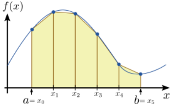
Note that $a = x_0$ and $b=x_{N}$. By using the familiar formula for the area of each trapezium, we can approximate the integral as

$$\begin{align}\mathcal{I}^{\mathrm{trapz}} &= \sum_{n=0}^{N-1} \Delta x \left(\frac{f(x_n) + f(x_{n+1})}{2}\right) \\ &= \Delta x \left[\left(\frac{f(x_0) + f(x_1)}{2}\right)+ \left(\frac{f(x_1) + f(x_2)}{2}\right) + \cdots + \left(\frac{f(x_{N-1}) + f(x_{N})}{2}\right)\right] \\ &= \Delta x \left[\frac{f(x_0)}{2} + \left(\sum_{n=1}^{N-1} f(x_n)\right) + \frac{f(x_{N})}{2}\right].\end{align}$$

9.2.1 Python Implementation of the Trapezium Rule

In Scipy, the trapezium rule is implemented by the trapz function. It usually takes two array arguments, y and x; then the function call trapz(y,x) returns the trapezium rule estimate for $\int y \;dx$, using the elements of x as the discretization points, and the elements of y as the values of the integrand at those points.

Note

Matlab compatibility note: Be careful of the order of inputs! For the Scipy function, it's trapz(y,x). For the Matlab function of the same name, the inputs are supplied in the opposite order, as trapz(x,y).

Note that the discretization points in x need not be equally-spaced. Alternatively, you can call the function as trapz(y,dx=s); this performs the numerical integration assuming equally-spaced discretization points, with spacing s.

Here is an example of using trapz to evaluate the integral $\int_0^\infty \exp(-x^2) dx = 1$:

>>> from scipy import *
>>> x = linspace(0,10,25)
>>> y = exp(-x)
>>> t = trapz(y,x)
>>> print(t)
1.01437984777

9.2.2 Numerical Error for the Trapezium Rule

From a visual comparison of Fig. 9.1.1 (for the mid-point rule) and Fig. $\PageIndex{1}$ (for the trapezium rule), we might be tempted to conclude that the trapezium rule should be more accurate. Before jumping to that conclusion, however, let's do the actual calculation of the numerical error. This is similar to our above calculation of the mid-point rule's numerical error. For the trapezium rule, however, it's convenient to consider a pair of adjacent segments, which lie between the three discretization points $\left\{x_{n-1}, x_n, x_{n+1}\right\}$.

As before, we perform a Taylor expansion of $f(x)$ in the vicinity of $x_{n}$:

$$f(x) = f(x_n) + f'(x_n) (x-x_n) + \frac{f''(x_n)}{2} (x-x_n)^2 + \frac{f'''(x_n)}{6} (x-x_n)^3 + \cdots$$

If we integrate $f(x)$ from $x_{n-1}$ to $x_{n+1}$, the result is

$$\begin{align} \mathcal{I}_n & \equiv \int_{x_n - \Delta x}^{x_n + \Delta x} f(x) dx \\ &= \; 2 f(x_n) \Delta x \;\;+\; f'(x_n) \int_{x_n - \Delta x}^{x_n + \Delta x} (x-x_n) dx \; +\; \frac{f''(x_n)}{2} \int_{x_n - \Delta x}^{x_n + \Delta x} (x-x_n)^2 dx \; +\; \cdots \end{align}$$

As before, every other term on the right-hand side integrates to zero. We are left with

$$\mathcal{I}_n \; = \; 2 f(x_n) \Delta x \;+\; \frac{f''(x_n)}{3} \Delta x^3 + O(\Delta x^5) \;+\; \cdots$$

This has to be compared to the estimate produced by the trapezium rule, which is

$$\mathcal{I}_n^{\mathrm{(trapz)}} = \Delta x \left[ \frac{f(x_{n-1})}{2} + f(x_n) + \frac{f(x_{n+1})}{2}\right].$$

If we Taylor expand the first and last terms of the above expression around $x_{n}$, the result is:

$$\begin{align} \mathcal{I}_n^{\mathrm{(trapz)}} & = \frac{\Delta x}{2} \left[f(x_n) - f'(x_n) \Delta x + \frac{f''(x_n)}{2} \Delta x^2 - \frac{f'''(x_n)}{6} \Delta x^3 + \frac{f''''(x_n)}{24} \Delta x^4 + O(\Delta x^4)\right] \\ &\quad + \;\;\Delta x \; f(x_n) \\ &\quad + \frac{\Delta x}{2} \left[f(x_n) + f'(x_n) \Delta x + \frac{f''(x_n)}{2} \Delta x^2 + \frac{f'''(x_n)}{6} \Delta x^3 + \frac{f''''(x_n)}{24} \Delta x^4 + O(\Delta x^4)\right] \\ & = 2 f(x_n) \Delta x + \frac{f''(x_n)}{2} \Delta x^3 + O(\Delta x^5). \end{align}$$

Hence, the numerical error for integrating over this pair of segments is

$$\mathcal{E}_n \;\equiv\; \left|\mathcal{I}_n - \mathcal{I}_n^{\mathrm{trapz}}\right| \;=\; \frac{|f''(x_n)|}{6} \Delta x^3 \;\sim\; O\left(\frac{1}{N^3}\right).$$

And the total numerical error goes as

$$\mathcal{E}_{\mathrm{total}} \sim O\left(\frac{1}{N^2}\right),$$

which is the same scaling as the mid-point rule! Despite our expectations, the trapezium rule isn't actually an improvement over the mid-point rule, as far as numerical accuracy is concerned.