Computers: Solving the Pendulum

INTRODUCTION

The physical pendulum treated within a Hamiltonian formulation is a natural topic for study in a course in advanced classical mechanics. For the past three years we have been offering a series of problem sets studying this system numerically in our third year undergraduate courses.

Our computational physics is based on Mathematica¹ with some C communicating with Mathematica, although nothing in the body of the paper below is dependent on that choice. We have nonetheless found this system, and particularly its graphics, to be a good one for use with undergraduates. Some information on the hardware/software of our facility and the implementation of this package is provided in the Appendix.

Our work with our students has focused on two main areas: (I) investigation of the physics of the pendulum; and (II) exploration of various forms of Runge-Kutta algorithms to solve Hamilton’s equations. Initially these were both discussed in our mechanics course; the second has now been split off into a separate offering on computational physics at the third year undergraduate level. Both are described below.

A crucial question for this sort of application is how to prevent the students from becoming mired in the details of a computing environment. Our facility provides a locally written menu system that allows the students to edit and run Mathematica program files without ever having to know a file name or directory structure; although other approaches are available to our students, the overwhelming majority of them find this environment to be the most convenient. We supply a written tutorial of about seven pages on ways to use our locally written packages on the pendulum; with this plus a small amount of classroom time, most students complete their problem sets with minimal supervision.

By the time they reach their third year of studies our students have already used our computing facility, although usually not the numerical methods component of it that is the foundation of the work described here. Early in their first year they take a required computerized test on error analysis.² A variety of fitters, graphers, etc. are available in support of our laboratory program; this usage is optional but the overwhelming majority of our students regularly use these tools.^3,4 In their second year they write a required, nearly-trivial program in Mathematica. Some students have made extensive but non-required use of our Mathematica environment and/or taken courses in the Department of Computer Science. For most, however, this is their first serious exposure to this part of our computing environment. Thus, it is fair to say that at the beginning of this work our students have little of no knowledge of Mathematica.

Each of the two projects described below are designed to take roughly six hours of computer connect time to be completed. In the first project the students work in pairs, while in the second they work alone. The second project is also supported by over one hour of formal lectures on the theory of Runge-Kutta and other integrators of differential equations. Although we observe fairly large variations among our students, we seem to have ‘dialed in’ the requirements fairly realistically.

I. THE PHYSICS OF THE PENDULUM

The technology allows the students to calculate a time series of position momentum pairs in a matter of seconds; it is this fact that allows them to engage in a series of what if explorations. The students are encouraged to treat these problem sets as a series of experiments in which the result is unknown until the data is calculated. We typically ask the students to calculate on the order of 1000 points using a supplied fourth-order Runge-Kutta.

Using the non-dimensional Hamiltonian:

\[H (q,p) = \frac{p^2}{2} + (1–cosq) \tag{1}\]

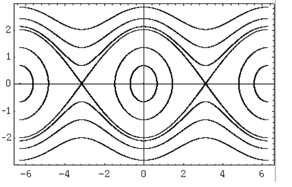
we first ask the students to produce a number of such time series (7 or so) for q₀ = 0 and π, and p₀ ranging evenly from -2 to +2 (including p₀ = 0). Plotting the phase portrait of all of these on a single graph allows them to develop a geometric as opposed to an algebraic understanding of the dynamics. Figure 1 shows some sample output. The students first identify the separatrices which divide the phase space into regions of closed and open orbits, corresponding physically to oscillations and rotations of the pendulum. The region inside the separatrices has a "bowl shaped" geometry around the fixed point (or equilibrium state) at the center; this implies that the fixed point is nonlinearly stable. The region near the fixed point where the separatrices cross has a "saddle shaped" geometry, implying that it is unstable.

Although there is nothing revolutionary about such plots when they appear in textbooks,⁵ we believe the ability of the student to produce them from their own initial conditions in a few minutes makes a valuable educational impact not possible by looking at a figure in a book.

We then turn our attention to a system that we do not think could be discussed at all in this course without our computational facility: the physical pendulum with the support point oscillating sinusoidally in the vertical direction. This system is not solvable analytically, and exhibits both chaotic as well as non-chaotic behavior. The ‘perturbed’ Hamiltonian is:

\[H (q,p) = \frac{p^2}{2} + (1+hcos\gamma t)(1–cosq) \tag{2}\]

We supply a package which returns solutions for user-specified initial conditions and parameters which are Poincare´ sections, ie: position-momentum pairs for every gravitational period t = t₀ + 2mπ/γ (where m is an integer), rather than every time step. Thus the sections are time ‘slices’ of the three dimensional (q,p,t) extended phase space.

In a Poincare´ section chaotic solutions are visible as clouds of points, while non-chaotic solutions are visible as closed curves. The closed curves correspond to tori in the extended phase space.

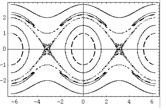
We lead students to discover that for h << 1 the separatrices of the unperturbed pendulum break up into regions of chaos, while the closed curves around the stable fixed point of the unperturbed pendulum are only slightly deformed. Figure 2 shows a typical graph. The students are asked to explore how the width of the chaotic region depends on h for a fixed value of γ.

The students find values of h and γ for which there are secondary tori that do not encircle the origin. Once found, producing Poincare´ sections for values t₀ = 0,π/(2γ),π/γ,3π/(2γ) leads to an understanding of the topology of the extended phase space.

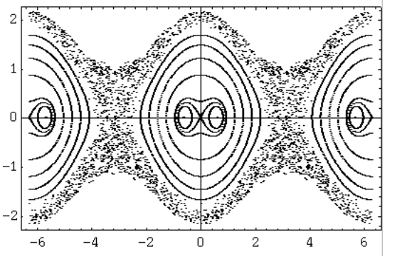
We also study parametric resonance, which occurs when the frequency γ or one of its harmonics is close to twice the natural frequency of the pendulum. This destabilizes the fixed point q = 0, p = 0, and is what makes it possible to swing on a swing. Figure 3 shows an example. The Poincare´ sections allow a determination of the limits of instability and their dependence on h, which can be directly compared with perturbation theory

Finally, we have the students demonstrate that for γ >> 1 the perturbation stabilizes the fixed point q = π, p = 0, which is unstable in the unperturbed system. The value of γ for which this occurs can be determined and compared with theoretical values.

II. RUNGE-KUTTA ALGORITHMS

The other aspect of our work on the pendulum is an investigation of the Runge-Kutta algorithm being used to solve the equations of motion for the unperturbed case. As mentioned above, this work originally occurred in our course in classical mechanics but has now been split off into a separate offering on computational physics.

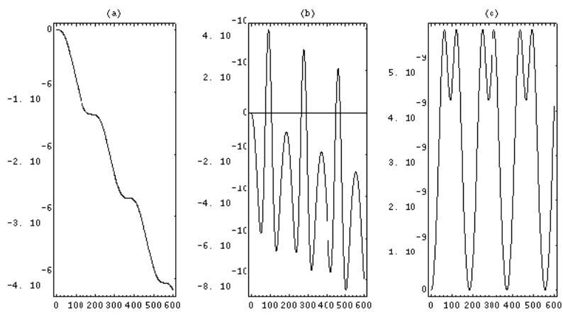
We provide the students with code to choose the order of the RungeKutta to be 1 (Euler), 2, 3, 4, 5 or a symplectic algorithm for the unperturbed pendulum.⁶ We measure the accuracy of the computation by the degree to which the calculated energy is conserved. Figure 4 show some sample output.

The symplectic algorithm is an area-preserving (ie. Hamiltonian) discretization of the dynamics. We particularly like the fact that this algorithm is suggested by the physics of the problem, not the numerical methods.

For speed reasons the actual integrator is coded in C communicating with Mathematica. In the first year of this problem set we provided the students with the code for a fourth-order Runge-Kutta and asked them to modify that code to produce lower order integrators. Despite the fact that the modification involved mostly removing code, this was much too difficult for many of our students and was in general a disaster. In the second year of the project we coded all orders and asked the students to choose the order by modifying a C pre-processor #define appearing prominently near the top of the C file. This works well. An advantage of this approach is that the program is displayed by the editor used to modify the define; students who are so inclined may examine it to see how the program works, while others at least have the program in front of them as they hunt for the pre-processor directive.

We then ask our students to calculate a time series for a closed orbit that covers several tens of periods, and take the Fourier transform of the position. In addition to the usual questions of side bands and aliases, we have the students use the central frequency to calculate the period and compare it to the exact value, as given by:⁷

\[T = 2\sqrt{2} \int_0^Q \frac{dq}{(cosq – cosQ)^{1/2}} \tag{3}\]

where Q is the maximum amplitude. Naturally, we ask the students to evaluate the integral in software; included in this is a comparison of Mathematica’s built-in numerical integrator with a direct numerical evaluation using a repeated midpoint rule. We finally ask the students to investigate experimentally how the sharpness of the central peak depends on the size of the timestep ∆t used in the computation.

III. CONCLUSIONS

We have been pleased with the contribution these projects have made to the learning of our students. Both formal and informal assessments by the students confirm our impressions: the students are aware of the pedagogical value of this work and, further, seem to have had a great deal of fun in completing it.

A possible criticism of our work is that the material discussed above in §II is fairly computeresque for a course in classical mechanics, which is where it was for the first two years. Although we tend to feel that exposing physics specialists to some details of computational physics is almost always worthwhile, the fact is that we used our students as ‘beta testers’ of this material for two years because we knew that our new course in computational physics was to be added to the curriculum.

We conclude with a caution. We had on the order of 40 students doing these assignments each academic year. Since we use a single multiuser/multitasking UNIX computer and X-terminals, we find that if the hardware/software is not capable of producing, say, a 1000 point time series in under five seconds of cpu or so, then when many students are trying to do their work the system backs up exponentially, leading to great frustration. We were fortunate to have been able to significantly upgrade the power of our facility after the first year; otherwise we would have been forced to ask considerably less of our students than what is described above.

Experience with both this work and other assignments for our students has led us to the formulation of the five seconds of cpu rule: if a quantum of computation cannot be completed in this period of time, then it is likely that we are making the students ask too much of the facility. The rule would not hold for workstations or multiple PC’s, and would depend on the number of X-terminals in use; we have 25 student X-terminals.

ACKNOWLEDGEMENTS

As is so often the case, it is our students who suffered through some of our mistakes; we hope their learning compensates in some measure for their frustration, and we thank them for their patience. The level of computing described here would have been impossible without the donation of our central compute server, a Hewlett-Packard 9000/750, by Hewlett-Packard (Canada) Ltd., whose support we gratefully acknowledge. The other members of the UPSCALE group in the Department have been very generous with their time for discussion and advice about this project; they are Richard C. Bailey, James R. Drummond, R. Nigel Edwards, William R. Peltier, John M. Pitre and Pekka Sinervo. The symplectic integrator was coded by Djoko Wirosoetisno.

APPENDIX

We have based much of our advanced undergraduate computing on Mathematica under UNIX, with X-terminals as our primary display device. Here we discuss some of the reasons for our software/hardware decisions, and some of the implications.

The choice between Mathematica and Maple is a fairly religious topic which we will avoid here; there are also proponents of other similar software systems. Using one of these as a foundation for an undergraduate computing system is attractive for a number of reasons. Foremost is their symbolic algebra capability, although for a pedagogical application their excellent graphics capabilities are also crucial. The fact that they are interpreted encourages our students to engage in exploration, since they need not declare variable names or do a separate compile step to see the results of a calculation. This choice also neatly sidesteps the C versus FORTRAN wars that continue to rage in most physics departments.

For the work described here, we found that Runge-Kuttas coded directly in Mathematica were much too slow. Thus, we coded the actual integrators in C, which then communicates with Mathematica. Our experience is that without considerable support our students are not capable of working with C directly, although programming Mathematica (and presumably Maple) is quite within their reach.

Ease of administration is one of the main advantages of a UNIX/X-terminal hardware configuration; running multiple workstations and/or PC’s sounds very unattractive to one of us (DMH) who is responsible for system administration of our facility. Since our students spend a lot of their computer time ‘chewing on their pencil’ we can get away with many more X-terminals for a given compute-server than would be possible for power users like graduate students. This means that our cost per seat is comparatively low; nonetheless a powerful computer is in the ‘engine room’ for those times when it is required.

Finally, we all tend to conceive of software projects such as that described here without adequately calculating the time involved. The effort behind the work described here is non-trivial. Including false starts, bug fixes, supporting documentation, etc. we probably have about five person months invested in this. Our code and documentation are available on request; in addition these materials are available on the MathSource archive maintained by Wolfram Research.⁸

REFERENCES

1. Wolfram Research Inc., Mathematica (Wolfram Research, 1993) Version 2.2.

2. D. Harrison and J.M. Pitre, Phys. Teacher 21, 588 (1983).

3. D. Harrison and J.M. Pitre, Phys. Teacher 26, 156 (1988).

4. D. Harrison and J.M. Pitre, Comput. in Educ. 12, 261 (1988).

5. For example H. Goldstein, Classical Mechanics (Addison-Wesley, 1950), p. 290.

6. Runge-Kuttas are probably discussed in every book on numerical methods. For the less well known symplectic integrator see R. Ruth, IEEE Trans. Nucl Sci. 30, 2669 (1983), which formed the basis for our code.

7. For example I. Percival and D. Richards, Introduction to Dynamics (Cambridge Univ. Press, 1982), p. 57.

8. The code and documentation are item number 0206-109 on the MathSource archive. One simple way to retrieve the materials is to send a mail message stating Send 0206-109 to [e-mail].

Figure Captions

Figure 1: Momentum p versus angle q for the pendulum. Each time series consists of 1500 points with a time step of .02. The initial conditions are q₀ = 0 and π, and –2 ≤ p₀ ≤ 2 in steps of 2/3. Every point is "doubled" as (q, p) and (q ±2π,p).

Figure 2: Poincare´ section for the perturbed pendulum, illustrating integrable and chaotic behavior. Each time series consists 600 points, and the time step is .02. The initial conditions are (q₀,p₀) = (π,0.1), (π,1),(π,–1), (π,2),(π,–2), (π/2,0), (0,1), (0,2.2), and (0,–2.2). The time series is constructed by sampling the system every period, 2π/γ, and the amplitude and frequency of the perturbation are h = 0.1 and γ = 1.6 respectively.

Figure 3: Poincare´ sections for the perturbed pendulum, illustrating parametric resonance. The amplitude and frequency of the perturbation are h = 0.1 and γ = 2. The initial conditions are (q₀,p₀) = (0.0001+nπ/10,0) for n = 0, 1, 2, ... , 10. Each time series consists of 600 points, and the time step is 0.02.

Figure 4: Plotting E-1 versus time step for the unperturbed pendulum. The initial conditions are q₀ = π/2, p₀ = 0, and we have calculated 600 time steps each of size .02. If the calculation conserved energy perfectly, E would be exactly one.

a. Third-order Runge-Kutta.

b. Fourth-order Runge-Kutta.

c. Symplectic algorithm (fourth-order accurate).