6.4: Fermi’s Golden Rule

We consider now a system with an Hamiltonian $\mathcal{H}_{0}$, of which we know the eigenvalues and eigenfunctions:

$$\mathcal{H}_{0} u_{k}(x)=E_{k} u_{k}(x)=\hbar \omega_{k} u_{k}(x) \nonumber$$

Here I just expressed the energy eigenvalues in terms of the frequencies $\omega_{k}=E_{k} / \hbar$. Then, a general state will evolve as:

$$\psi(x, t)=\sum_{k} c_{k}(0) e^{-i \omega_{k} t} u_{k}(x) \nonumber$$

If the system is in its equilibrium state, we expect it to be stationary, thus the wavefunction will be one of the eigenfunctions of the Hamiltonian. For example, if we consider an atom or a nucleus, we usually expect to find it in its ground state (the state with the lowest energy). We consider this to be the initial state of the system:

$$\psi(x, 0)=u_{i}(x) \nonumber$$

where $i$ stands for initial ). Now we assume that a perturbation is applied to the system. For example, we could have a laser illuminating the atom, or a neutron scattering with the nucleus. This perturbation introduces an extra potential $\hat{V}$ in the system’s Hamiltonian (a priori $\hat{V}$ can be a function of both position and time $\hat{V}(x, t)$, but we will consider the simpler case of time-independent potential $\hat{V}(x)$). Now the hamiltonian reads:

$$\mathcal{H}=\mathcal{H}_{0}+\hat{V}(x) \nonumber$$

What we should do, is to find the eigenvalues $\left\{E_{h}^{v}\right\}$ and eigenfunctions $\left\{v_{h}(x)\right\}$ of this new Hamiltonian and express $u_{i}(x)$ in this new basis and see how it evolves:

$$u_{i}(x)=\sum_{h} d_{h}(0) v_{h} \quad \rightarrow \quad \psi^{\prime}(x, t)=\sum_{h} d_{h}(0) e^{-i E_{h}^{v} t / \hbar} v_{h}(x). \nonumber$$

Most of the time however, the new Hamiltonian is a complex one, and we cannot calculate its eigenvalues and eigenfunctions. Then we follow another strategy.

Consider the examples above (atom+laser or nucleus+neutron): What we want to calculate is the probability of making a transition from an atom/nucleus energy level to another energy level, as induced by the interaction. Since $\mathcal{H}_{0}$ is the original Hamiltonian describing the system, it makes sense to always describe the state in terms of its energy levels (i.e. in terms of its eigenfunctions). Then, we guess a solution for the state of the form:

$$\psi^{\prime}(x, t)=\sum_{k} c_{k}(t) e^{-i \omega_{k} t} u_{k}(x) \nonumber$$

This is very similar to the expression for $\psi(x, t)$ above, except that now the coefficient $c_{k}$ are time dependent. The time-dependency derives from the fact that we added an extra potential interaction to the Hamiltonian.

Let us now insert this guess into the Schrödinger equation, $i \hbar \frac{\partial \psi^{\prime}}{\partial t}=\mathcal{H}_{0} \psi^{\prime}+\hat{V} \psi^{\prime}$:

$$i \hbar \sum_{k}\left[\dot{c}_{k}(t) e^{-i \omega_{k} t} u_{k}(x)-i \omega c_{k}(t) e^{-i \omega_{k} t} u_{k}(x)\right]=\sum_{k} c_{k}(t) e^{-i \omega_{k} t}\left(\mathcal{H}_{0} u_{k}(x)+\hat{V}\left[u_{k}(x)\right]\right) \nonumber$$

(where $\dot{c}$ is the time derivative). Using the eigenvalue equation to simplify the RHS we find

$$\sum_{k}\left[i \hbar \dot{c}_{k}(t) e^{-i \omega_{k} t} u_{k}(x)\right. \left.+\hbar \omega c_{k}(t) e^{-i \omega_{k} t} u_{k}(x)\right]= \sum_{k}\left[c_{k}(t) e^{-i \omega_{k} t} \hbar \omega_{k} u_{k}(x)+\right. \left.c_{k}(t) e^{-i \omega_{k} t} \hat{V}\left[u_{k}(x)\right]\right] \nonumber$$

$$\sum_{k} i \hbar \dot{c}_{k}(t) e^{-i \omega_{k} t} u_{k}(x)=\sum_{k} c_{k}(t) e^{-i \omega_{k} t} \hat{V}\left[u_{k}(x)\right] \nonumber$$

Now let us take the inner product of each side with $u_{h}(x)$:

$$\sum_{k} i \hbar \dot{c}_{k}(t) e^{-i \omega_{k} t} \int_{-\infty}^{\infty} u_{h}^{*}(x) u_{k}(x) d x=\sum_{k} c_{k}(t) e^{-i \omega_{k} t} \int_{-\infty}^{\infty} u_{h}^{*}(x) \hat{V}\left[u_{k}(x)\right] d x \nonumber$$

In the LHS we find that $\int_{-\infty}^{\infty} u_{h}^{*}(x) u_{k}(x) d x=0$ for $h \neq k$ and it is 1 for $h = k$ (the eigenfunctions are orthonormal). Then in the sum over $k$ the only term that survives is the one $k = h$:

$$\sum_{k} i \hbar \dot{c}_{k}(t) e^{-i \omega_{k} t} \int_{-\infty}^{\infty} u_{h}^{*}(x) u_{k}(x) d x=i \hbar \dot{c}_{h}(t) e^{-i \omega_{h} t} \nonumber$$

On the RHS we do not have any simplification. To shorten the notation however, we call $V_{h k}$ the integral:

$$V_{h k}=\int_{-\infty}^{\infty} u_{h}^{*}(x) \hat{V}\left[u_{k}(x)\right] d x \nonumber$$

The equation then simplifies to:

$$\dot{c}_{h}(t)=-\frac{i}{\hbar} \sum_{k} c_{k}(t) e^{i\left(\omega_{h}-\omega_{k}\right) t} V_{h k} \nonumber$$

This is a differential equation for the coefficients $c_{h}(t)$. We can express the same relation using an integral equation:

$$c_{h}(t)=-\frac{i}{\hbar} \sum_{k} \int_{0}^{t} c_{k}\left(t^{\prime}\right) e^{i\left(\omega_{h}-\omega_{k}\right) t^{\prime}} V_{h k} d t^{\prime}+c_{h}(0) \nonumber$$

We now make an important approximation. We said at the beginning that the potential $\hat{V}$ is a perturbation, thus we assume that its effects are small (or the changes happen slowly). Then we can approximate $c_{k}\left(t^{\prime}\right)$ in the integral with its value at time 0, $c_{k}(t=0)$:

$$c_{h}(t)=-\frac{i}{\hbar} \sum_{k} c_{k}(0) \int_{0}^{t} e^{i\left(\omega_{h}-\omega_{k}\right) t^{\prime}} V_{h k} d t^{\prime}+c_{h}(0) \nonumber$$

[Notice: for a better approximation, an iterative procedure can be used which replaces $c_{k}\left(t^{\prime}\right)$ with its first order solution, then second etc.].

Now let’s go back to the initial scenario, in which we assumed that the system was initially at rest, in a stationary state $\psi(x, 0)=u_{i}(x)$. This means that $c_{k}(0)=0$ for all $k \neq i$. The equation then reduces to:

$$c_{h}(t)=-\frac{i}{\hbar} \int_{0}^{t} e^{i\left(\omega_{h}-\omega_{i}\right) t^{\prime}} V_{h i} d t^{\prime} \nonumber$$

or, by calling $\Delta \omega_{h}=\omega_{h}-\omega_{i}$,

$$c_{h}(t)=-\frac{i}{\hbar} V_{h i} \int_{0}^{t} e^{i \Delta \omega_{h} t^{\prime}} d t^{\prime}=-\frac{V_{h i}}{\hbar \Delta \omega_{h}}\left(1-e^{i \Delta \omega_{h} t}\right) \nonumber$$

What we are really interested in is the probability of making a transition from the initial state $u_{i}(x)$ to another state $u_{h}(x): P(i \rightarrow h)=\left|c_{h}(t)\right|^{2}$. This transition is caused by the extra potential $\hat{V}$ but we assume that both initial and final states are eigenfunctions of the original Hamiltonian $\mathcal{H}_{0}$ (notice however that the final state will be a superposition of all possible states to which the system can transition to).

We obtain

$$P(i \rightarrow h)=\frac{4\left|V_{h i}\right|^{2}}{\hbar^{2} \Delta \omega_{h}^{2}} \sin \left(\frac{\Delta \omega_{h} t}{2}\right)^{2} \nonumber$$

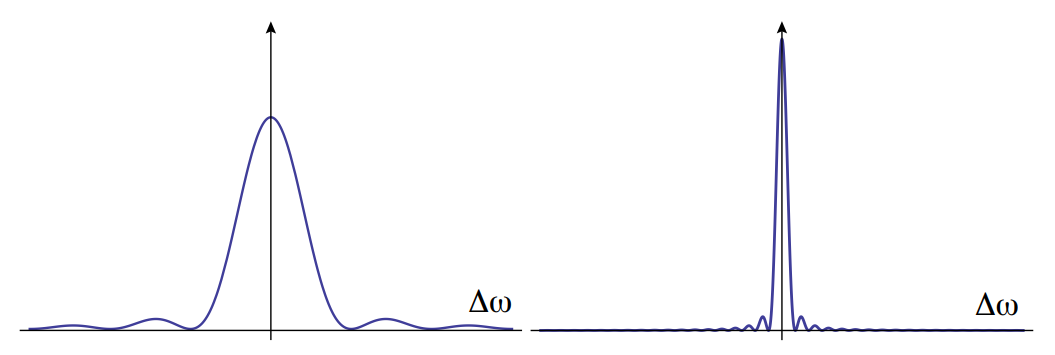
The function $\frac{\sin z}{z}$ is called a sinc function (see Figure $\PageIndex{1}$). Take $\frac{\sin (\Delta \omega t / 2)}{\Delta \omega / 2}$. In the limit $t \rightarrow \infty$ (i.e. assuming we are describing the state of the system after the new potential has had a long time to change the state of the quantum system) the sinc function becomes very narrow, until when we can approximate it with a delta function. The exact limit of the function gives us:

$$P(i \rightarrow h)=\frac{2 \pi\left|V_{h i}\right|^{2} t}{\hbar^{2}} \delta\left(\Delta \omega_{h}\right) \nonumber$$

We can then find the transition rate from $i \rightarrow h$ as the probability of transition per unit time, $W_{i h}=\frac{d P(i \rightarrow h)}{d t}$:

$$\boxed{W_{i h}=\frac{2 \pi}{\hbar^{2}}\left|V_{h i}\right|^{2} \delta\left(\Delta \omega_{h}\right)} \nonumber$$

This is the so-called Fermi’s Golden Rule, describing the transition rate between states.

Obs.

This transition rate describes the transition from $u_{i}$ to a single level $u_{h}$ with a given energy $E_{h}=\hbar \omega_{h}$. In many cases the final state is an unbound state, which, as we saw, can take on a continuous of possible energy available. Then, instead of the point-like delta function, we consider the transition to a set of states with energies in a small interval $E \rightarrow E+d E$. The transition rate is then proportional to the number of states that can be found with this energy. The number of state is given by $d n=\rho(E) d E$, where $\rho(E)$ is called the density of states (we will see how to calculate this in a later lecture). Then, Fermi’s Golden rule is more generally expressed as:

$$\boxed{W_{i h}=\left.\frac{2 \pi}{\hbar}\left|V_{h i}\right|^{2} \rho\left(E_{h}\right)\right|_{E_{h}=E_{i}}} \nonumber$$

[Note, before making the substitution $\delta(\Delta \omega) \rightarrow \rho(E)$ we need to write $\delta(\Delta \omega)=\hbar \delta(\hbar \Delta \omega)=\hbar \delta\left(E_{h}-E_{i}\right) \rightarrow \left.\hbar \rho\left(E_{h}\right)\right|_{E_{h}=E_{i}}$. This is why in the final formulation for the Golden rule we only have a factor $\hbar$ and not its square.]

Figure $\PageIndex{1}$: Sinc function $\frac{\sin (\Delta \omega t / 2)}{\Delta \omega / 2}$. Left: Sinc function at short times. Right: Sinc function at longer times, the function becoming narrower and closer to a Dirac delta function (CC BY-NC-ND; Paola Cappellaro)