Physics LibreTexts

2.10: Designing an Achromatic Doublet

  • Page ID
    8303
  • \( \newcommand{\vecs}[1]{\overset { \scriptstyle \rightharpoonup} {\mathbf{#1}} } \)

    \( \newcommand{\vecd}[1]{\overset{-\!-\!\rightharpoonup}{\vphantom{a}\smash {#1}}} \)

    \( \newcommand{\id}{\mathrm{id}}\) \( \newcommand{\Span}{\mathrm{span}}\)

    ( \newcommand{\kernel}{\mathrm{null}\,}\) \( \newcommand{\range}{\mathrm{range}\,}\)

    \( \newcommand{\RealPart}{\mathrm{Re}}\) \( \newcommand{\ImaginaryPart}{\mathrm{Im}}\)

    \( \newcommand{\Argument}{\mathrm{Arg}}\) \( \newcommand{\norm}[1]{\| #1 \|}\)

    \( \newcommand{\inner}[2]{\langle #1, #2 \rangle}\)

    \( \newcommand{\Span}{\mathrm{span}}\)

    \( \newcommand{\id}{\mathrm{id}}\)

    \( \newcommand{\Span}{\mathrm{span}}\)

    \( \newcommand{\kernel}{\mathrm{null}\,}\)

    \( \newcommand{\range}{\mathrm{range}\,}\)

    \( \newcommand{\RealPart}{\mathrm{Re}}\)

    \( \newcommand{\ImaginaryPart}{\mathrm{Im}}\)

    \( \newcommand{\Argument}{\mathrm{Arg}}\)

    \( \newcommand{\norm}[1]{\| #1 \|}\)

    \( \newcommand{\inner}[2]{\langle #1, #2 \rangle}\)

    \( \newcommand{\Span}{\mathrm{span}}\) \( \newcommand{\AA}{\unicode[.8,0]{x212B}}\)

    \( \newcommand{\vectorA}[1]{\vec{#1}}      % arrow\)

    \( \newcommand{\vectorAt}[1]{\vec{\text{#1}}}      % arrow\)

    \( \newcommand{\vectorB}[1]{\overset { \scriptstyle \rightharpoonup} {\mathbf{#1}} } \)

    \( \newcommand{\vectorC}[1]{\textbf{#1}} \)

    \( \newcommand{\vectorD}[1]{\overrightarrow{#1}} \)

    \( \newcommand{\vectorDt}[1]{\overrightarrow{\text{#1}}} \)

    \( \newcommand{\vectE}[1]{\overset{-\!-\!\rightharpoonup}{\vphantom{a}\smash{\mathbf {#1}}}} \)

    \( \newcommand{\vecs}[1]{\overset { \scriptstyle \rightharpoonup} {\mathbf{#1}} } \)

    \( \newcommand{\vecd}[1]{\overset{-\!-\!\rightharpoonup}{\vphantom{a}\smash {#1}}} \)

    \(\newcommand{\avec}{\mathbf a}\) \(\newcommand{\bvec}{\mathbf b}\) \(\newcommand{\cvec}{\mathbf c}\) \(\newcommand{\dvec}{\mathbf d}\) \(\newcommand{\dtil}{\widetilde{\mathbf d}}\) \(\newcommand{\evec}{\mathbf e}\) \(\newcommand{\fvec}{\mathbf f}\) \(\newcommand{\nvec}{\mathbf n}\) \(\newcommand{\pvec}{\mathbf p}\) \(\newcommand{\qvec}{\mathbf q}\) \(\newcommand{\svec}{\mathbf s}\) \(\newcommand{\tvec}{\mathbf t}\) \(\newcommand{\uvec}{\mathbf u}\) \(\newcommand{\vvec}{\mathbf v}\) \(\newcommand{\wvec}{\mathbf w}\) \(\newcommand{\xvec}{\mathbf x}\) \(\newcommand{\yvec}{\mathbf y}\) \(\newcommand{\zvec}{\mathbf z}\) \(\newcommand{\rvec}{\mathbf r}\) \(\newcommand{\mvec}{\mathbf m}\) \(\newcommand{\zerovec}{\mathbf 0}\) \(\newcommand{\onevec}{\mathbf 1}\) \(\newcommand{\real}{\mathbb R}\) \(\newcommand{\twovec}[2]{\left[\begin{array}{r}#1 \\ #2 \end{array}\right]}\) \(\newcommand{\ctwovec}[2]{\left[\begin{array}{c}#1 \\ #2 \end{array}\right]}\) \(\newcommand{\threevec}[3]{\left[\begin{array}{r}#1 \\ #2 \\ #3 \end{array}\right]}\) \(\newcommand{\cthreevec}[3]{\left[\begin{array}{c}#1 \\ #2 \\ #3 \end{array}\right]}\) \(\newcommand{\fourvec}[4]{\left[\begin{array}{r}#1 \\ #2 \\ #3 \\ #4 \end{array}\right]}\) \(\newcommand{\cfourvec}[4]{\left[\begin{array}{c}#1 \\ #2 \\ #3 \\ #4 \end{array}\right]}\) \(\newcommand{\fivevec}[5]{\left[\begin{array}{r}#1 \\ #2 \\ #3 \\ #4 \\ #5 \\ \end{array}\right]}\) \(\newcommand{\cfivevec}[5]{\left[\begin{array}{c}#1 \\ #2 \\ #3 \\ #4 \\ #5 \\ \end{array}\right]}\) \(\newcommand{\mattwo}[4]{\left[\begin{array}{rr}#1 \amp #2 \\ #3 \amp #4 \\ \end{array}\right]}\) \(\newcommand{\laspan}[1]{\text{Span}\{#1\}}\) \(\newcommand{\bcal}{\cal B}\) \(\newcommand{\ccal}{\cal C}\) \(\newcommand{\scal}{\cal S}\) \(\newcommand{\wcal}{\cal W}\) \(\newcommand{\ecal}{\cal E}\) \(\newcommand{\coords}[2]{\left\{#1\right\}_{#2}}\) \(\newcommand{\gray}[1]{\color{gray}{#1}}\) \(\newcommand{\lgray}[1]{\color{lightgray}{#1}}\) \(\newcommand{\rank}{\operatorname{rank}}\) \(\newcommand{\row}{\text{Row}}\) \(\newcommand{\col}{\text{Col}}\) \(\renewcommand{\row}{\text{Row}}\) \(\newcommand{\nul}{\text{Nul}}\) \(\newcommand{\var}{\text{Var}}\) \(\newcommand{\corr}{\text{corr}}\) \(\newcommand{\len}[1]{\left|#1\right|}\) \(\newcommand{\bbar}{\overline{\bvec}}\) \(\newcommand{\bhat}{\widehat{\bvec}}\) \(\newcommand{\bperp}{\bvec^\perp}\) \(\newcommand{\xhat}{\widehat{\xvec}}\) \(\newcommand{\vhat}{\widehat{\vvec}}\) \(\newcommand{\uhat}{\widehat{\uvec}}\) \(\newcommand{\what}{\widehat{\wvec}}\) \(\newcommand{\Sighat}{\widehat{\Sigma}}\) \(\newcommand{\lt}{<}\) \(\newcommand{\gt}{>}\) \(\newcommand{\amp}{&}\) \(\definecolor{fillinmathshade}{gray}{0.9}\)

    It is not the intention of this chapter to study lens aberrations. However, the design of an achromatic doublet lens lends itself to the sort of calculation we are doing in this chapter.

    A combination of two lenses in contact, a converging lens made of crown glass and a weaker diverging lens made of flint glass, can be designed so that the combination is a converging lens that is almost achromatic. Flint glass is a little denser than crown glass, and has a higher refractive index and a greater dispersive power.

    The dispersive power \(\omega\) of glass is usually defined as

    \[\omega= \frac{n^{(F)}-n^{(C)}}{n^{(D)}-1}.\label{eq:2.10.1} \]

    Here C, D and F refer to the wavelengths of the C, D and F Fraunhofer lines in the solar spectrum, which are respectively, H\(\alpha\) (656.3 nm), Na I (589.3 nm), H\(\beta\) (486.1 nm), and which may be loosely referred to as “red”, “yellow” and “blue”. A typical value for a crown glass would be about 0.016, and a typical value for a flint glass would be about 0.028.

    An achromatic doublet is typically made of a positive crown glass lens whose power is positive but which decreases with increasing wavelength (i.e. toward the red), cemented to a weaker flint glass lens whose power is negative and also decreases (in magnitude) with increasing wavelength. The sum of the two powers is positive, and varies little with wavelength, going through a shallow minimum. Typically, in designing an achromatic doublet, there will be two requirements to be satisfied: 1. The power or focal length in yellow will be specified, and 2. You would like the power in red to be the same as the power in blue, and to vary little in between.

    Consider the doublet illustrated in Figure II.15, constructed of a biconvex crown lens and a biconcave flint lens.
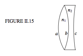
    FIGURE II.15.png

    I have indicated the indices and the radii of curvature. The power (reciprocal of the focal length) of the first lens by itself is

    \[ P_1 = (n_1-1) \left(\frac{1}{a}+\frac{1}{b}\right),\label{eq:2.10.2} \]

    and the power of the second lens is

    \[ P_2 = -(n_2-1)\left( \frac{1}{b}+\frac{1}{c}\right). \label{eq:2.10.3} \]

    I shall write these for short, in obvious notation, as

    \[ P_1 = k_1(n_1-1), \qquad P_2 = -k_2(n_2-1). \label{eq:2.10.4a,b} \]

    But we need equations like these for each of the three wavelengths, thus:

    \[ P_1^{(C)} = k_1(n_1^{(C)}-1), \qquad P_2^{(C)} = -k_2(n_2^{(C)}-1), \label{eq:2.10.5a,b} \]

    \[ P_1^{(D)} = k_1(n_1^{(D)}-1), \qquad P_2^{(D)} = -k_2(n_2^{(D)}-1),\label{eq:2.10.6a,b} \]

    \[P_1^{(F)} = k_1(n_1^{(F)}-1), \qquad P_2^{(F)} = -k_2(n_2^{(F)}-1). \label{eq:2.10.7a,b} \]

    Now we want to satisfy two conditions. One is that the total power be specified:

    \[P_1^{(D)} +P_2^{(D)} = P^{(D)} . \label{eq:2.10.8} \]

    The other is that the total power in the red is to equal the total power in the blue, and I now make use of equations \(\ref{eq:2.10.5a,b}\) and \(\ref{eq:2.10.7a,b}\):

    \[ k_1(n^{(C)}_1- 1) - k_2(n^{(C)}_2-1)= k_1(n^{(F)}_1- 1) - k_2(n^{(F)}_2-1).\label{eq:2.10.9} \]

    On rearrangement, this becomes

    \[ k_1(n^{(F)}_1- n^{(C)}_1) = k_2(n^{(F)}_2-n^{(C)}_2). \label{eq:2.10.10} \]

    Now, making use of equations \(\ref{eq:2.10.1}\) and \(\ref{eq:2.10.6a,b}\), we obtain the condition that the powers will be the same in red and blue:

    \[ \omega_1P_1 + \omega_2 P_2 = 0. \label{eq:2.10.11} \]

    For example, suppose that we want the focal length in yellow to be 16 cm ( \(P^{(D)}= 0.0625\) cm-1) and that the dispersive powers are 0.016 and 0.028. Equations \(\ref{eq:2.10.8}\) and \(\ref{eq:2.10.11}\) then tell us that we must have \( P_1^{(D)}= 0.14583\) cm-1 \) and \(P_2^{(D)}= -0.083\) cm-1. (\(f_1 =6.86\) cm and \(f_2 = -12.0\) cm).

    If we want to make the first lens equibiconvex, so that \(a = b\), and if \(n_1 = 1.5\), Equation \(\ref{eq:2.10.2}\) tells us that \(a\) = 6.86 cm. If \(n_2 = 1.6\), Equation \(\ref{eq:2.10.3}\) then tells us that \(c = −144\) cm. That \(c\) is negative tells us that our assumption that the flint lens was concave to the right was wrong; it is convex to the right.

    Exercise \(\PageIndex{1}\)

    Suppose that, instead of making the crown lens equibiconvex, you elect to make the last surface flat – i.e. \(c\) = ∞. What, then, must \(a\) and \(b\) be?

    Answers. \(a\) = 6.55 cm, \(b\) = 7.20 cm.


    This page titled 2.10: Designing an Achromatic Doublet is shared under a CC BY-NC 4.0 license and was authored, remixed, and/or curated by Jeremy Tatum via source content that was edited to the style and standards of the LibreTexts platform.

    • Was this article helpful?