2.14: Exercise
- Page ID
- 8307
\( \newcommand{\vecs}[1]{\overset { \scriptstyle \rightharpoonup} {\mathbf{#1}} } \)
\( \newcommand{\vecd}[1]{\overset{-\!-\!\rightharpoonup}{\vphantom{a}\smash {#1}}} \)
\( \newcommand{\dsum}{\displaystyle\sum\limits} \)
\( \newcommand{\dint}{\displaystyle\int\limits} \)
\( \newcommand{\dlim}{\displaystyle\lim\limits} \)
\( \newcommand{\id}{\mathrm{id}}\) \( \newcommand{\Span}{\mathrm{span}}\)
( \newcommand{\kernel}{\mathrm{null}\,}\) \( \newcommand{\range}{\mathrm{range}\,}\)
\( \newcommand{\RealPart}{\mathrm{Re}}\) \( \newcommand{\ImaginaryPart}{\mathrm{Im}}\)
\( \newcommand{\Argument}{\mathrm{Arg}}\) \( \newcommand{\norm}[1]{\| #1 \|}\)
\( \newcommand{\inner}[2]{\langle #1, #2 \rangle}\)
\( \newcommand{\Span}{\mathrm{span}}\)
\( \newcommand{\id}{\mathrm{id}}\)
\( \newcommand{\Span}{\mathrm{span}}\)
\( \newcommand{\kernel}{\mathrm{null}\,}\)
\( \newcommand{\range}{\mathrm{range}\,}\)
\( \newcommand{\RealPart}{\mathrm{Re}}\)
\( \newcommand{\ImaginaryPart}{\mathrm{Im}}\)
\( \newcommand{\Argument}{\mathrm{Arg}}\)
\( \newcommand{\norm}[1]{\| #1 \|}\)
\( \newcommand{\inner}[2]{\langle #1, #2 \rangle}\)
\( \newcommand{\Span}{\mathrm{span}}\) \( \newcommand{\AA}{\unicode[.8,0]{x212B}}\)
\( \newcommand{\vectorA}[1]{\vec{#1}} % arrow\)
\( \newcommand{\vectorAt}[1]{\vec{\text{#1}}} % arrow\)
\( \newcommand{\vectorB}[1]{\overset { \scriptstyle \rightharpoonup} {\mathbf{#1}} } \)
\( \newcommand{\vectorC}[1]{\textbf{#1}} \)
\( \newcommand{\vectorD}[1]{\overrightarrow{#1}} \)
\( \newcommand{\vectorDt}[1]{\overrightarrow{\text{#1}}} \)
\( \newcommand{\vectE}[1]{\overset{-\!-\!\rightharpoonup}{\vphantom{a}\smash{\mathbf {#1}}}} \)
\( \newcommand{\vecs}[1]{\overset { \scriptstyle \rightharpoonup} {\mathbf{#1}} } \)
\(\newcommand{\longvect}{\overrightarrow}\)
\( \newcommand{\vecd}[1]{\overset{-\!-\!\rightharpoonup}{\vphantom{a}\smash {#1}}} \)
\(\newcommand{\avec}{\mathbf a}\) \(\newcommand{\bvec}{\mathbf b}\) \(\newcommand{\cvec}{\mathbf c}\) \(\newcommand{\dvec}{\mathbf d}\) \(\newcommand{\dtil}{\widetilde{\mathbf d}}\) \(\newcommand{\evec}{\mathbf e}\) \(\newcommand{\fvec}{\mathbf f}\) \(\newcommand{\nvec}{\mathbf n}\) \(\newcommand{\pvec}{\mathbf p}\) \(\newcommand{\qvec}{\mathbf q}\) \(\newcommand{\svec}{\mathbf s}\) \(\newcommand{\tvec}{\mathbf t}\) \(\newcommand{\uvec}{\mathbf u}\) \(\newcommand{\vvec}{\mathbf v}\) \(\newcommand{\wvec}{\mathbf w}\) \(\newcommand{\xvec}{\mathbf x}\) \(\newcommand{\yvec}{\mathbf y}\) \(\newcommand{\zvec}{\mathbf z}\) \(\newcommand{\rvec}{\mathbf r}\) \(\newcommand{\mvec}{\mathbf m}\) \(\newcommand{\zerovec}{\mathbf 0}\) \(\newcommand{\onevec}{\mathbf 1}\) \(\newcommand{\real}{\mathbb R}\) \(\newcommand{\twovec}[2]{\left[\begin{array}{r}#1 \\ #2 \end{array}\right]}\) \(\newcommand{\ctwovec}[2]{\left[\begin{array}{c}#1 \\ #2 \end{array}\right]}\) \(\newcommand{\threevec}[3]{\left[\begin{array}{r}#1 \\ #2 \\ #3 \end{array}\right]}\) \(\newcommand{\cthreevec}[3]{\left[\begin{array}{c}#1 \\ #2 \\ #3 \end{array}\right]}\) \(\newcommand{\fourvec}[4]{\left[\begin{array}{r}#1 \\ #2 \\ #3 \\ #4 \end{array}\right]}\) \(\newcommand{\cfourvec}[4]{\left[\begin{array}{c}#1 \\ #2 \\ #3 \\ #4 \end{array}\right]}\) \(\newcommand{\fivevec}[5]{\left[\begin{array}{r}#1 \\ #2 \\ #3 \\ #4 \\ #5 \\ \end{array}\right]}\) \(\newcommand{\cfivevec}[5]{\left[\begin{array}{c}#1 \\ #2 \\ #3 \\ #4 \\ #5 \\ \end{array}\right]}\) \(\newcommand{\mattwo}[4]{\left[\begin{array}{rr}#1 \amp #2 \\ #3 \amp #4 \\ \end{array}\right]}\) \(\newcommand{\laspan}[1]{\text{Span}\{#1\}}\) \(\newcommand{\bcal}{\cal B}\) \(\newcommand{\ccal}{\cal C}\) \(\newcommand{\scal}{\cal S}\) \(\newcommand{\wcal}{\cal W}\) \(\newcommand{\ecal}{\cal E}\) \(\newcommand{\coords}[2]{\left\{#1\right\}_{#2}}\) \(\newcommand{\gray}[1]{\color{gray}{#1}}\) \(\newcommand{\lgray}[1]{\color{lightgray}{#1}}\) \(\newcommand{\rank}{\operatorname{rank}}\) \(\newcommand{\row}{\text{Row}}\) \(\newcommand{\col}{\text{Col}}\) \(\renewcommand{\row}{\text{Row}}\) \(\newcommand{\nul}{\text{Nul}}\) \(\newcommand{\var}{\text{Var}}\) \(\newcommand{\corr}{\text{corr}}\) \(\newcommand{\len}[1]{\left|#1\right|}\) \(\newcommand{\bbar}{\overline{\bvec}}\) \(\newcommand{\bhat}{\widehat{\bvec}}\) \(\newcommand{\bperp}{\bvec^\perp}\) \(\newcommand{\xhat}{\widehat{\xvec}}\) \(\newcommand{\vhat}{\widehat{\vvec}}\) \(\newcommand{\uhat}{\widehat{\uvec}}\) \(\newcommand{\what}{\widehat{\wvec}}\) \(\newcommand{\Sighat}{\widehat{\Sigma}}\) \(\newcommand{\lt}{<}\) \(\newcommand{\gt}{>}\) \(\newcommand{\amp}{&}\) \(\definecolor{fillinmathshade}{gray}{0.9}\)Exercise \(\PageIndex{1}\)
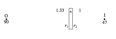
An object is placed 90 cm to the left of a thin lens in air. The image is real and is 99 cm to the right of the lens.
However, if the medium to the right of the lens is water (refractive index 1.33), the image is virtual and is 76 cm to the left of the lens.
And if the medium to the left of the lens is water (and to the right is air) the image is real and 47 cm to the right of the lens.
Calculate the two radii of curvature and the refractive index of the glass.
Exercise \(\PageIndex{2}\)
An object is placed 100 cm to the left of the first surface (A) of a thick lens (thickness = 10 cm) in air. The image is real and is 25 cm to the right of the second surface (B).
However, if the medium to the right of the second surface (B) is water (refractive index 1.33), the image is real and 41 cm to the right of surface B.
And if the medium to the left of surface A is water (and to the right of B is air) the image is real and 92 cm to the right of the lens.
Calculate the two radii of curvature and the refractive index of the glass.
Neither of these two problems is likely to turn up in a practical situation – but they are very good practice for difficult lens problems! Solutions on the next page – but no peeking until you have tried them!
Solutions
1. First:

\[\frac{1}{99} = -{1}{90} +\frac{n-1}{r_1}+\frac{1-n}{r_2}.\label{eq:2.14.1} \]
Second:

\[-\frac{-1.33}{76}=-\frac{1}{90}+\frac{n-1}{r_1}+\frac{1.33-n}{r_2}. \label{eq:2.14.2} \]
(You might be tempted to think that the left hand side of this equation should be \(\frac{1}{76}\). Make sure that you understand why this is wrong.)
Third:

\[\frac{1}{47} = -\frac{1.33}{90}+\frac{n-1.33}{r_1}+\frac{1-n}{r_2}.\label{eq:2.14.3} \]
The physics is now finished. All that has to be done is to solve the three equations for the three unknowns. I would start by letting \( x=r_1, y=r_2, z = n\). The equations then become:
\[z(x-y)-x+y=0.021212121,\label{eq:2.14.4} \]
\[z(x − y) − x + 1.33 y = − 0.006388889 \label{eq:2.14.5} \]
and
\[z(x − y) − 1.33 x + y = 0.036054374.\label{eq:2.14.6} \]
These are easy to solve:
\(x= − 0.044977, \quad y = − 0.083639, \quad z = + 1.54864.\)
Thus
\(r_1 = 22.23 \text{cm},\qquad r_2 = 11.96 \text{cm},\qquad n=1.5549 \text{cm} \)
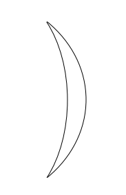
The lens is a positive meniscus lens (i.e. thicker in the middle), both surfaces being convex to the right. It looks like this:

2.
First:

\[C_1 = -\frac{1}{100}\label{eq:2.14.7} \]
\[C_2 = -\frac{1}{100} + \frac{n-1}{r_1} = \frac{100n-100-r_1}{100r_1}\label{eq:2.14.8} \]
\[C_3 = \frac{nC_2}{n-10C_2} = \frac{100n^2 - 100n-r_1n}{100r_1n+10r_1 - 1000n + 1000}\label{eq:2.14.9} \]
\[ C_4 = \frac{100n^2-100n - r_1n}{100r_1n+10r_1-1000n+1000}+\frac{1-n}{r_2}=\frac{1}{25}\label{eq:2.14.10} \]
Second:

\[C_1 = -\frac{1}{100}\label{eq:2.14.11} \]
\[C_2 = -\frac{1}{100}+\frac{n-1}{r_1} = \frac{100n-100-r_1}{100r_1}\label{eq:2.14.12} \]
\[C_3 = \frac{nC_2}{n-10C_2}=\frac{100n^2-100n-r_1n}{100r_1n+10r_1-1000n+1000}\label{eq:2.14.13} \]
\[C_4= \frac{100n^2-100n-r_1n}{100r_1n+10r_1-1000n+1000}+\frac{1.33-n}{r_2} =\frac{1.33}{41}\label{eq:2.14.14} \]
So far, we have obtained two complicated-looking Equations (\(\ref{eq:2.14.10}\) and \(\ref{eq:2.14.14\)) in the three unknowns \(r_1, r_2\) and \(n\), and we are just about to embark on obtaining a third equation from the third experiment, after which we shall have to face the unpleasant task of solving the three equations. But look! – before we press on, we may discover that we can already solve for \(r_2\) from Equations \(\ref{eq:2.14.10}\) and \(\ref{eq:2.14.14}\). I make it
\[r_2 = - 43.645 161 29 \text{cm}\label{eq:2.14.15} \]
so that the second surface is concave to the left – i.e. it bulges towards the right. This was an unexpected piece of good fortune! We can now move on to the third experiment.
Third:

\[C_1 = -\frac{1.33}{100}\label{eq:2.14.16} \]
\[C_2 = -\frac{1.33}{100 }+\frac{n-1.33}{r_1}=\frac{100n-133-1.33r_1}{100r_1}\label{eq:2.14.17} \]
\[C_3 = \frac{nC_2}{n-10C_2}=\frac{100n^2-133n-1.33r_1n}{100r_1n+13.3r_1-1000n+1330}\label{eq:2.14.18} \]
\[C_4= \frac{100n^2-133n-1.33r_1n}{100r_1n+13.3r_1 -1000n + 1300}+\frac{1-n}{r_2} = \frac{1}{92}\label{eq:2.14.19} \]
We can now solve Equations \(\ref{eq:2.14.10}\) and \(\ref{eq:2.14.19}\), or \(\ref{eq:2.14.14}\) and \(\ref{eq:2.14.19}\) for \(r_1\) and \(n\). The very conscientious will want to solve them using \(\ref{eq:2.14.10}\) and \(\ref{eq:2.14.19}\) and then repeat the solution using \(\ref{eq:2.14.14}\) and \(\ref{eq:2.14.19}\), and verify that they give the same answer, and will then further verify that the correct solutions have been obtained by substitution in each of the three equations in turn. Being slightly less conscientious, I am going to use Equations \(\ref{eq:2.14.10}\) and \(\ref{eq:2.14.19}\), and I shall then verify that the solutions obtained satisfy Equation \(\ref{eq:2.14.14}\).
I find it easier to solve equations in \(x\) and \(y\) rather than in \(r_1\) and \(n\), so I am going to let \(x = r_1\) and \(y = n\). Then, bearing in mind that we have already found that \( r_2 = -43.645 161 29\), Equations \(\ref{eq:2.14.10}\) and \(\ref{eq:2.14.19}\) become, respectively, after a little algebra and arithmetic,
\[\frac{100y^2 -100y -xy}{100xy+10x-1000y+1000} = by +c \label{eq:2.14.20} \]
and
\[\frac{100y^2-100ay-axy}{100xy+10ax-1000y+1000a}=by+d,\label{eq:2.14.21} \]
where
a = +1.33
b = -0.02291204730
c = +0.06291204630
d =+0.03379161252
After a little more slightly tedious but routine algebra and arithmetic, these become
\[Axy^2 +By^2 + C_1xy + D_1x+E_1y+ F_1 = 0\label{eq:2.14.22} \]
and
\[Axy^2 + By^2+C_2xy+D_2x+E^2y+F_2 = 0, \label{eq:2.14.23} \]
where
A = 2.291204730
B = 77.08795270
C1 = -7.062084 257
D1 = -0.6291204730
E1 = -14.17590540
F1 = -62.91204730
C2 = -4.403431023
D2 = -0.449295447
E2 = -68.74536457
F2 = -44.92954465.
Then we have to solve these two equations! These can be solved, for example, by the method described in Section 1.9 of Chapter 1 of the notes on Celestial Mechanics. Since I already have a computer program that does that, I used it and got \(x = 15.386908\) and \(y = .1 518865\). Thus the solution for the lens is
\( r_1 = + 15.39 \text{cm} \qquad r_2 = -43.65 \text{cm} \qquad n = 1.519\)
The first surface is convex to the left, and the second surface is convex to the right. I.e. the lens is “fat”, bulging in the middle.
As a check that our arithmetic is all right, we can verify that this solution also satisfies Equation \( \ref{eq:2.14.14}\). (It does!)
As a further check, the reader might now like to start with these numbers, and an object distance of 100 cm, and see if it results in the three image distances given in the original problem. (It does!)
Another way to solve equations \( \ref{eq:2.14.22}\) and \( \ref{eq:2.14.23}\) is to subtract the former from the latter to obtain
\[axy+bx+cy +d =0, \label{eq:2.14.24} \]
when
\(a\) = 2.658653234
\(b\) = 0.179825026
\(c\) = -54.56945917
\(d\) = 17.98260265.
You can then express \(x\) and a function of \(y\) and substitute into Equation \( \ref{eq:2.14.22}\) (or into \( \ref{eq:2.14.23}\), or both as a check). You then have a single cubic equation in \(y\), rather than two simultaneous equations in \(x\) and \(y\), as follows:
\[(Ba-Ac_y^3+(E_1a+Bb-C_1c-Ad)y^2+(F_1a+E_1b-D_1c-C_1d)y+F_1b-D_1c =0.\label{eq:2.14.25} \]
Numerically, this is
\[329.9799377y^3- 450.4024164y^2 - 77.14660950y - 6.294\times10^{-5} =0. \label{eq:2.14.26} \]
The only positive real root of this is \(y (= n) = 1.518864\), which is the same as we obtained before. The value of \(x (= r_1)\) is then readily found, from Equation \(\ref{eq:2.14.24}\), to be 15.3869 cm, as before.
Exercise \(\PageIndex{3}\)
A converging lens has a focal length of 40 cm in air. What is its focal length when it is immersed in water, of refractive index 1.333?
After a moment’s thought you will demand that you be told the refractive index of the glass. After further thought, you will conclude that not only do you need to know the refractive index of the glass, but you also need to know the shape (radii of curvature of the surfaces) of the lens.
So, here’s the question properly set.
A biconvex lens is made of glass of refractive index 1.5. The radii of curvature of its surfaces are 25 cm and 100 cm. What is its focal length in air? What would be its focal length if immersed in water of refractive index 4/3? What would be its focal length if immersed in carbon bisulphide of refractive index 5/3?
Exercise \(\PageIndex{4}\)
A lens has a focal length in air of 30 cm.
A block of glass with the same refractive index as the above lens has an air bubble inside it of exactly the same size and shape of the above lens. What is the focal length of this lens-shaped bubble?
You may be asking yourself if you need to know the shape of the lens, or the refractive index of the glass. I’ll let you ponder.
Exercise \(\PageIndex{5}\)
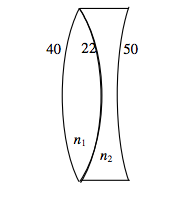
A thin cemented doublet is made of two thin lenses cemented together, as shown in the drawing below. The radii of curvature in cm are indicated in the drawing. The refractive index of the left hand lens is \(n_1\), and that of the right hand lens is \(n_2\). The combination results in an overall diverging doublet lens of focal length 127 cm.

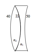
As a result of a manufacturing error, the two types of glass are inadvertently exchanged, and a doublet lens as shown below is made:

This combination results in an overall converging doublet lens of focal lens 72 cm. Calculate the refractive indices of the two types of glass.
Here are my solutions to problems 3 to 5
Solutions
3. The focal length in air is given by
\(\frac{}{} = 0 +\frac{1.5-1.0}{25} + \frac{1.0-1.5}{-100}, \qquad \text{whence} \underline{\underline{f = 40 \text{cm}}} \)
The focal length in water is given by
\( \frac{\frac{4}{3}}{f} = 0 + \frac{\frac{3}{2}-\frac{4}{3}}{25} + \frac{\frac{4}{3}-\frac{3}{2}}{-100}, \qquad \text{whence} \underline{\underline{f = 160 \text{cm}}}\)
The focal length in CS2 is given by
\(\frac{\frac{5}{3}}{f} = 0 + \frac{\frac{3}{2}-\frac{5}{3}}{25}+\frac{\frac{5}{3}-\frac{3}{2}}{-100}, \qquad \text{whence} \underline{\underline{f = -200 \text{cm}}} \)
4. Regardless of the shape of the lens, the focal length of the glass lens in air is given by
\( \frac{1}{f_{\text{lens}}}= (n-1) \left(\frac{1}{r_1}-\frac{1}{r_2}\right),\)
whereas the focal length of the bubble in glass is given by
\(\frac{1}{f_{\text{bubble}}}= (n-1) \left(\frac{1}{r_1}-\frac{1}{r_2}\right).\)
Thus
\(\underline{\underline{f_\text{bubble} = -n \times f_\text{lens} = -30n \quad \text{cm}}}\)
5. The focal lengths of the two doublets are related to the refractive indices by
\( -\frac{1}{127}= \frac{n_1-1}{40} +\frac{n_2-n_2}{-22}+\frac{1-n_2}{50}\)
and
\(\frac{1}{72} = \frac{n_2-1}{40}+\frac{n_1-n_2}{-22}+\frac{1-n_1}{50}\)
These equations can be rewritten
\( 1968n_1-18288n_2 + 803 = 0 \)
and
\(1296n_1 -1395n_2 + 374 = 0,\)
with solutions
\(\underline{\underline{ n_1 = 1.521 \qquad n_2= 1.682}}\)


