
1.1: Experimental motivations
- Page ID
- 57539

\( \newcommand{\vecs}[1]{\overset { \scriptstyle \rightharpoonup} {\mathbf{#1}} } \)
\( \newcommand{\vecd}[1]{\overset{-\!-\!\rightharpoonup}{\vphantom{a}\smash {#1}}} \)
\( \newcommand{\dsum}{\displaystyle\sum\limits} \)
\( \newcommand{\dint}{\displaystyle\int\limits} \)
\( \newcommand{\dlim}{\displaystyle\lim\limits} \)
\( \newcommand{\id}{\mathrm{id}}\) \( \newcommand{\Span}{\mathrm{span}}\)
( \newcommand{\kernel}{\mathrm{null}\,}\) \( \newcommand{\range}{\mathrm{range}\,}\)
\( \newcommand{\RealPart}{\mathrm{Re}}\) \( \newcommand{\ImaginaryPart}{\mathrm{Im}}\)
\( \newcommand{\Argument}{\mathrm{Arg}}\) \( \newcommand{\norm}[1]{\| #1 \|}\)
\( \newcommand{\inner}[2]{\langle #1, #2 \rangle}\)
\( \newcommand{\Span}{\mathrm{span}}\)
\( \newcommand{\id}{\mathrm{id}}\)
\( \newcommand{\Span}{\mathrm{span}}\)
\( \newcommand{\kernel}{\mathrm{null}\,}\)
\( \newcommand{\range}{\mathrm{range}\,}\)
\( \newcommand{\RealPart}{\mathrm{Re}}\)
\( \newcommand{\ImaginaryPart}{\mathrm{Im}}\)
\( \newcommand{\Argument}{\mathrm{Arg}}\)
\( \newcommand{\norm}[1]{\| #1 \|}\)
\( \newcommand{\inner}[2]{\langle #1, #2 \rangle}\)
\( \newcommand{\Span}{\mathrm{span}}\) \( \newcommand{\AA}{\unicode[.8,0]{x212B}}\)
\( \newcommand{\vectorA}[1]{\vec{#1}} % arrow\)
\( \newcommand{\vectorAt}[1]{\vec{\text{#1}}} % arrow\)
\( \newcommand{\vectorB}[1]{\overset { \scriptstyle \rightharpoonup} {\mathbf{#1}} } \)
\( \newcommand{\vectorC}[1]{\textbf{#1}} \)
\( \newcommand{\vectorD}[1]{\overrightarrow{#1}} \)
\( \newcommand{\vectorDt}[1]{\overrightarrow{\text{#1}}} \)
\( \newcommand{\vectE}[1]{\overset{-\!-\!\rightharpoonup}{\vphantom{a}\smash{\mathbf {#1}}}} \)
\( \newcommand{\vecs}[1]{\overset { \scriptstyle \rightharpoonup} {\mathbf{#1}} } \)
\(\newcommand{\longvect}{\overrightarrow}\)
\( \newcommand{\vecd}[1]{\overset{-\!-\!\rightharpoonup}{\vphantom{a}\smash {#1}}} \)
\(\newcommand{\avec}{\mathbf a}\) \(\newcommand{\bvec}{\mathbf b}\) \(\newcommand{\cvec}{\mathbf c}\) \(\newcommand{\dvec}{\mathbf d}\) \(\newcommand{\dtil}{\widetilde{\mathbf d}}\) \(\newcommand{\evec}{\mathbf e}\) \(\newcommand{\fvec}{\mathbf f}\) \(\newcommand{\nvec}{\mathbf n}\) \(\newcommand{\pvec}{\mathbf p}\) \(\newcommand{\qvec}{\mathbf q}\) \(\newcommand{\svec}{\mathbf s}\) \(\newcommand{\tvec}{\mathbf t}\) \(\newcommand{\uvec}{\mathbf u}\) \(\newcommand{\vvec}{\mathbf v}\) \(\newcommand{\wvec}{\mathbf w}\) \(\newcommand{\xvec}{\mathbf x}\) \(\newcommand{\yvec}{\mathbf y}\) \(\newcommand{\zvec}{\mathbf z}\) \(\newcommand{\rvec}{\mathbf r}\) \(\newcommand{\mvec}{\mathbf m}\) \(\newcommand{\zerovec}{\mathbf 0}\) \(\newcommand{\onevec}{\mathbf 1}\) \(\newcommand{\real}{\mathbb R}\) \(\newcommand{\twovec}[2]{\left[\begin{array}{r}#1 \\ #2 \end{array}\right]}\) \(\newcommand{\ctwovec}[2]{\left[\begin{array}{c}#1 \\ #2 \end{array}\right]}\) \(\newcommand{\threevec}[3]{\left[\begin{array}{r}#1 \\ #2 \\ #3 \end{array}\right]}\) \(\newcommand{\cthreevec}[3]{\left[\begin{array}{c}#1 \\ #2 \\ #3 \end{array}\right]}\) \(\newcommand{\fourvec}[4]{\left[\begin{array}{r}#1 \\ #2 \\ #3 \\ #4 \end{array}\right]}\) \(\newcommand{\cfourvec}[4]{\left[\begin{array}{c}#1 \\ #2 \\ #3 \\ #4 \end{array}\right]}\) \(\newcommand{\fivevec}[5]{\left[\begin{array}{r}#1 \\ #2 \\ #3 \\ #4 \\ #5 \\ \end{array}\right]}\) \(\newcommand{\cfivevec}[5]{\left[\begin{array}{c}#1 \\ #2 \\ #3 \\ #4 \\ #5 \\ \end{array}\right]}\) \(\newcommand{\mattwo}[4]{\left[\begin{array}{rr}#1 \amp #2 \\ #3 \amp #4 \\ \end{array}\right]}\) \(\newcommand{\laspan}[1]{\text{Span}\{#1\}}\) \(\newcommand{\bcal}{\cal B}\) \(\newcommand{\ccal}{\cal C}\) \(\newcommand{\scal}{\cal S}\) \(\newcommand{\wcal}{\cal W}\) \(\newcommand{\ecal}{\cal E}\) \(\newcommand{\coords}[2]{\left\{#1\right\}_{#2}}\) \(\newcommand{\gray}[1]{\color{gray}{#1}}\) \(\newcommand{\lgray}[1]{\color{lightgray}{#1}}\) \(\newcommand{\rank}{\operatorname{rank}}\) \(\newcommand{\row}{\text{Row}}\) \(\newcommand{\col}{\text{Col}}\) \(\renewcommand{\row}{\text{Row}}\) \(\newcommand{\nul}{\text{Nul}}\) \(\newcommand{\var}{\text{Var}}\) \(\newcommand{\corr}{\text{corr}}\) \(\newcommand{\len}[1]{\left|#1\right|}\) \(\newcommand{\bbar}{\overline{\bvec}}\) \(\newcommand{\bhat}{\widehat{\bvec}}\) \(\newcommand{\bperp}{\bvec^\perp}\) \(\newcommand{\xhat}{\widehat{\xvec}}\) \(\newcommand{\vhat}{\widehat{\vvec}}\) \(\newcommand{\uhat}{\widehat{\uvec}}\) \(\newcommand{\what}{\widehat{\wvec}}\) \(\newcommand{\Sighat}{\widehat{\Sigma}}\) \(\newcommand{\lt}{<}\) \(\newcommand{\gt}{>}\) \(\newcommand{\amp}{&}\) \(\definecolor{fillinmathshade}{gray}{0.9}\)By the beginning of the 1900s, physics (which by that time included what we now call nonrelativistic classical mechanics, classical thermodynamics and statistics, and classical electrodynamics including the geometric and wave optics) looked like an almost completed discipline, with most humanscale phenomena reasonably explained, and just a couple of mysterious "dark clouds"\(^{2}\) on the horizon. However, rapid technological progress and the resulting development of more refined scientific instruments have led to a fast multiplication of observed phenomena that could not be explained on a classical basis. Let me list the most consequential of those experimental findings.
(i) The blackbody radiation measurements, pioneered by G. Kirchhoff in 1859 , have shown that in the thermal equilibrium, the power of electromagnetic radiation by a fully absorbing ("black") surface, per unit frequency interval, drops exponentially at high frequencies. This is not what could be expected from the combination of classical electrodynamics and statistics, which predicted an infinite growth of the radiation density with frequency.
Indeed, classical electrodynamics shows \(^{3}\) that electromagnetic field modes evolve in time just as harmonic oscillators, and that the number \(d N\) of these modes in a large free-space volume \(V \gg \lambda^{3}\), within a small frequency interval \(d \omega<<\omega\) near some frequency \(\omega\), is
\[d N=2 V \frac{d^{3} k}{(2 \pi)^{3}}=2 V \frac{4 \pi k^{2} d k}{(2 \pi)^{3}}=V \frac{\omega^{2}}{\pi^{2} c^{3}} d \omega,\]
where \(c \approx 3 \times 10^{8} \mathrm{~m} / \mathrm{s}\) is the free-space speed of light, \(k=\omega / c\) the free-space wave number, and \(\lambda=2 \pi / k\) is the radiation wavelength. On the other hand, classical statistics \(^{4}\) predicts that in the thermal equilibrium at temperature \(T\), the average energy \(E\) of each 1D harmonic oscillator should be equal to \(k_{\mathrm{B}} T\), where \(k_{\mathrm{B}}\) is the Boltzmann constant. \(^{5}\) Combining these two results, we readily get the so-called Rayleigh-Jeans formula for the average electromagnetic wave energy per unit volume:
\[u \equiv \frac{1}{V} \frac{d E}{d \omega}=\frac{k_{\mathrm{B}} T}{V} \frac{d N}{d \omega}=\frac{\omega^{2}}{\pi^{2} c^{3}} k_{\mathrm{B}} T,\]
that diverges at \(\omega \rightarrow \infty\) (Fig. \(\PageIndex{1}\)) - the so-called ultraviolet catastrophe. On the other hand, the blackbody radiation measurements, improved by O. Lummer and E. Pringsheim, and also by H. Rubens and F. Kurlbaum to reach a \(1 \%\)-scale accuracy, were compatible with the phenomenological law suggested in 1900 by Max Planck:
\[u=\frac{\omega^{2}}{\pi^{2} c^{3}} \frac{\hbar \omega}{\exp \left\{\hbar \omega / k_{\mathrm{B}} T\right\}-1} .\]
This law may be reconciled with the fundamental Eq. (\(\PageIndex{1}\)) if the following replacement is made for the average energy of each field oscillator:
\[k_{\mathrm{B}} T \rightarrow \frac{\hbar \omega}{\exp \left(\hbar \omega / k_{\mathrm{B}} T\right)-1}\]
with a factor
\[\hbar \approx 1.055 \times 10^{-34} \mathrm{~J} \cdot \mathrm{s}\]
now called Planck’s constant. \({ }^{6}\) At low frequencies \(\left(\hbar \omega<<k_{\mathrm{B}} T\right)\), the denominator in Eq. (\(\PageIndex{3}\)) may be approximated as \(\hbar \omega / k_{\mathrm{B}} T\), so that the average energy (\(\PageIndex{4}\)) tends to its classical value \(k_{\mathrm{B}} T\), and the Planck’s law (3a) reduces to the Rayleigh-Jeans formula (2). However, at higher frequencies \((\hbar \omega>>\) \(k_{\mathrm{B}} T\) ), Eq. (\(\PageIndex{3}\)) describes the experimentally observed rapid decrease of the radiation density - see Fig. \(\PageIndex{1}\).
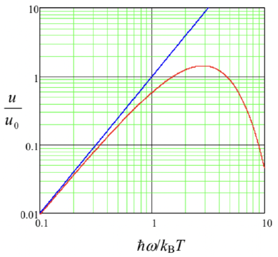
Fig. \(\PageIndex{1}\). The blackbody radiation density \(u\), in units of \(u_{0} \equiv\left(k_{\mathrm{B}} T\right)^{3} / \pi^{2} \hbar^{2} c^{3}\), as a function of frequency, according to the Rayleigh-Jeans formula (blue line) and the Planck’s law (red line).
M. Plank derived Eq. (\(\PageIndex{4}\)) from basic statistics, by assuming (just to fit the experimental results for u) that the energy of a field oscillator of frequency \(\omega\) can only take values that differ by (Energy vs frequency)
\[\ E=\hbar \omega,\]
(ii) The photoelectric effect, discovered in 1887 by H. Hertz and studied quantitatively by A. Stoletov in 1888-89, shows a sharp lower boundary ("red border") for the frequency of the incident light that may kick electrons out from metallic surfaces, independent of its intensity. Albert Einstein, in one of his three famous 1905 papers, noticed that this threshold \(\omega_{\min }\) could be explained by assuming that light consisted of certain particles (later called photons) with the same energy (\(\PageIndex{6}\)). \({ }^7\) Indeed, with this assumption, at the photon absorption by an electron, its energy \(E=\hbar \omega\) is divided between a fixed energy \(U_0\) (nowadays called the workfunction) of the electron's binding inside the metal, and the excess kinetic energy \(m_{\mathrm{e}} \nu^2 / 2>0\) of the freed electron - see Fig. \(\PageIndex{2}\). In this picture, the red border finds a natural explanation as \(\omega_{\min }=U_0 / \hbar .\(^{8}\)
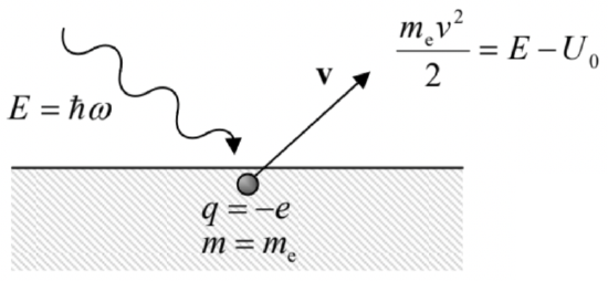 Fig. \(\PageIndex{2}\). Einstein’s explanation of the photoelectric effect’s frequency threshold.
(iii) The discrete frequency spectra of the electromagnetic radiation by excited atomic gases could not be explained by classical physics. (Applied to the planetary model of atoms, proposed by Ernst Rutherford, classical electrodynamics predicts the collapse of electrons on nuclei in \(\sim 10^{-10} \mathrm{~s}\), due to the electric-dipole radiation of electromagnetic waves. \({ }^{10}\) ) Especially challenging was the observation by Johann Jacob Balmer (in 1885) that the radiation frequencies of simple atoms may be well described by simple formulas. For example, for the lightest, hydrogen atom, all radiation frequencies may be numbered with just two positive integers \(n\) and \(n\) ’:
\[\omega_{n, n^{\prime}}=\omega_{0}\left(\frac{1}{n^{2}}-\frac{1}{n^{\prime 2}}\right),\]
with \(\omega_{0} \equiv \omega_{1, \infty} \approx 2.07 \times 10^{16} \mathrm{~s}^{-1}\). This observation, and the experimental value of \(\omega_{0}\), have found its first explanation in the famous 1913 theory by Niels Henrik David Bohr, which was a phenomenological precursor of the present-day quantum mechanics. In this theory, \(\omega_{n, n}\) ’ was interpreted as the frequency of a photon that obeys Einstein’s formula (5), with its energy \(E_{n, n^{\prime}}=\hbar \omega_{n . n^{\prime}}\) being the difference between two quantized (discrete) energy levels of the atom (Fig. \(\PageIndex{2}\)):
\[E_{n, n^{\prime}}=E_{n^{\prime}}-E_{n}>0 .\]
Bohr showed that Eq. (\(\PageIndex{7}\)) may be obtained from Eqs. (\(\PageIndex{6}\)) and (\(\PageIndex{8}\)), and non-relativistic \({ }^{11}\) classical mechanics, augmented with just one additional postulate, equivalent to the assumption that the angular momentum \(L=m_{\mathrm{e}} v r\) of an electron moving with velocity \(v\) on a circular orbit of radius \(r\) about the hydrogen’s nucleus (the proton, assumed to be at rest because of its much higher mass), is quantized as
\[L=\hbar n,\]
where \(\hbar\) is again the same Planck’s constant (Eq. \(\PageIndex{4}\)), and \(n\) is an integer. (In Bohr’s theory, \(n\) could not be equal to zero, though in the genuine quantum mechanics, it can.)
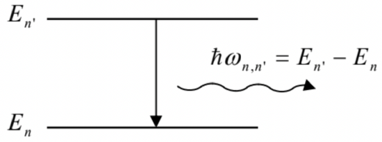
Fig. \(\PageIndex{3}\). The electromagnetic radiation of a system at a result of the transition between its quantized energy levels.
Indeed, it is sufficient to solve Eq. (\(\PageIndex{9}\)), \(m_{\mathrm{e}} v r=\hbar n\), together with the equation
\[m_{\mathrm{e}} \frac{v^{2}}{r}=\frac{e^{2}}{4 \pi \varepsilon_{0} r^{2}},\]
which expresses the \(2^{\text {nd }}\) Newton’s law for an electron rotating in the Coulomb field of the nucleus. (Here \(e \approx 1.6 \times 10^{-19} \mathrm{C}\) is the fundamental electric charge, and \(m_{\mathrm{e}} \approx 0.91 \times 10^{-30} \mathrm{~kg}\) is the electron’s rest mass.) The result for \(r\) is
\[r=n^{2} r_{\mathrm{B}}, \quad \text { where } r_{\mathrm{B}} \equiv \frac{\hbar^{2} / m_{\mathrm{e}}}{e^{2} / 4 \pi \varepsilon_{0}} \approx 0.0529 \mathrm{~nm} .\]
The constant \(r_{\mathrm{B}}\), called the Bohr radius, is the most important spatial scale of phenomena in atomic, molecular, and condensed-matter physics - and hence in all chemistry and biochemistry.
Now plugging these results into the non-relativistic expression for the full electron energy (with its rest energy taken for reference),
\[E=\frac{m_{\mathrm{e}} v^{2}}{2}-\frac{e^{2}}{4 \pi \varepsilon_{0} r},\]
we get the following simple expression for the electron’s energy levels:
\[E_{n}=-\frac{E_{\mathrm{H}}}{2 n^{2}}<0,\]
which, together with Eqs. (\(\PageIndex{6}\)) and (\(\PageIndex{8}\)), immediately gives Eq. (\(\PageIndex{7}\)) for the radiation frequencies. Here \(E_{\mathrm{H}}\) is called the so-called Hartree energy constant (or just the "Hartree energy") \({ }^{12}\) \[E_{\mathrm{H}} \equiv \frac{\left(e^{2} / 4 \pi \varepsilon_{0}\right)^{2}}{\hbar^{2} / m_{\mathrm{e}}} \approx 4.360 \times 10^{-18} \mathrm{~J} \approx 27.21 \mathrm{eV}\] (Note the useful relations, which follow from Eqs. (10) and (13a):
\[E_{\mathrm{H}}=\frac{e^{2}}{4 \pi \varepsilon_{0} r_{\mathrm{B}}}=\frac{\hbar^{2}}{m_{\mathrm{e}} r_{\mathrm{B}}^{2}}, \quad \text { i.e. } r_{\mathrm{B}}=\frac{e^{2} / 4 \pi \varepsilon_{0}}{E_{\mathrm{H}}}=\left(\frac{\hbar^{2} / m_{\mathrm{e}}}{E_{\mathrm{H}}}\right)^{1 / 2} ;\]
the first of them shows, in particular, that \(r_{\mathrm{B}}\) is the distance at which the natural scales of the electron’s potential and kinetic energies are equal.)
Note also that Eq. (\(\PageIndex{9}\)), in the form \(p r=\hbar n\), where \(p=m_{\mathrm{e}} v\) is the electron momentum’s magnitude, may be rewritten as the condition than an integer number \((n)\) of wavelengths \(\lambda\) of certain (before the late \(1920 \mathrm{~s}\), hypothetic) waves \(^{13}\) fits the circular orbit’s perimeter: \(2 \pi r \equiv 2 \pi \hbar n / p=n \lambda\). Dividing both parts of the last equality by \(n\), we see that for this statement to be true, the wave number \(k\) \(\equiv 2 \pi / \lambda\) of the de Broglie waves should be proportional to the electron’s momentum \(p=m v\) :
Momentum vs wave number \[\ p=\hbar k,\]
again with the same Planck’s constant as in Eq. (\(\PageIndex{6}\)).
(iv) The Compton effect \({ }^{14}\) is the reduction of frequency of X-rays at their scattering on free (or nearly-free) electrons - see Fig. \(\PageIndex{4}\) .
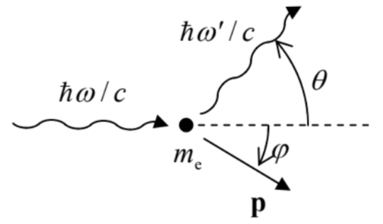 Fig. \(\PageIndex{4}\). The Compton effect.
The effect may be explained assuming that the X-ray photon also has a momentum that obeys the vector-generalized version of Eq. (\(\PageIndex{15}\)):
\[\mathbf{p}_{\text {photon }}=\hbar \mathbf{k}=\frac{\hbar \omega}{c} \mathbf{n},\]
where \(\mathbf{k}\) is the wavevector (whose magnitude is equal to the wave number \(k\), and whose direction coincides with the unit vector \(\mathbf{n}\) directed along the wave propagation \({ }^{15}\) ), and that the momenta of both the photon and the electron are related to their energies \(E\) by the classical relativistic formula \(^{16}\)
\[E^{2}=(c p)^{2}+\left(m c^{2}\right)^{2} .\]
(For a photon, the rest energy \(m\) is zero, and this relation is reduced to Eq. (\(\PageIndex{6}\)): \(E=c p=c \hbar k=\hbar \omega\).) Indeed, a straightforward solution of the following system of three equations,
\[\begin{aligned} \hbar \omega+m_{\mathrm{e}} c^{2} &=\hbar \omega^{\prime}+\left[(c p)^{2}+\left(m_{\mathrm{e}} c^{2}\right)^{2}\right]^{1 / 2}, \\ \frac{\hbar \omega}{c} &=\frac{\hbar \omega^{\prime}}{c} \cos \theta+p \cos \varphi, \\ 0 &=\frac{\hbar \omega^{\prime}}{c} \sin \theta-p \sin \varphi, \end{aligned}\]
(which express the conservation of, respectively, the full energy of the system and the two relevant Cartesian components of its full momentum, at the scattering event - see Fig. \(\PageIndex{4}\)), yields the result:
\[\frac{1}{\hbar \omega^{\prime}}=\frac{1}{\hbar \omega}+\frac{1}{m_{\mathrm{e}} c^{2}}(1-\cos \theta),\]
which is traditionally represented as the relation between the initial and final values of the photon’s wavelength \(\lambda=2 \pi / k=2 \pi /(\omega / c):{ }^{17}\)
[\lambda^{\prime}=\lambda+\frac{2 \pi \hbar}{m_{\mathrm{e}} c}(1-\cos \theta) \equiv \lambda+\lambda_{\mathrm{C}}(1-\cos \theta), \quad \text { with } \lambda_{\mathrm{C}} \equiv \frac{2 \pi \hbar}{m_{\mathrm{e}} c}\]
and is in agreement with experiment.
(v) De Broglie wave diffraction. In 1927, Clinton Joseph Davisson and Lester Germer, and independently George Paget Thomson succeeded to observe the diffraction of electrons on solid crystals (\(\PageIndex{5}\)). Specifically, they have found that the intensity of the elastic reflection of electrons from a crystal increases sharply when the angle \(\alpha\) between the incident beam of electrons and the crystal’s atomic planes, separated by distance \(d\), satisfies the following relation:
\[2 d \sin \alpha=n \lambda,\]
where \(\lambda=2 \pi / k=2 \pi \hbar / p\) is the de Broglie wavelength of the electrons, and \(n\) is an integer. As Fig. \(\PageIndex{5}\) shows, this is just the well-known condition \({ }^{18}\) that the path difference \(\Delta l=2 d \sin \alpha\) between the de Broglie waves reflected from two adjacent crystal planes coincides with an integer number of \(\lambda\), i.e. of the constructive interference of the waves. \({ }^{19}\)
To summarize, all the listed experimental observations could be explained starting from two very simple (and similarly looking) formulas: Eq. (\(\PageIndex{6}\)) (at that stage, for photons only), and Eq. (\(\PageIndex{16}\)) for both photons and electrons - both relations involving the same Planck’s constant. This fact might give an impression of experimental evidence sufficient to declare the light consisting of discrete particles (photons), and, on the contrary, electrons being some "matter waves" rather than particles. However, by that time (the mid-1920s), physics has accumulated overwhelming evidence of wave properties of light, such as interference and diffraction. \({ }^{20}\) In addition, there was also strong evidence for the lumped-particle ("corpuscular") behavior of electrons. It is sufficient to mention the famous oil-drop experiments by Robert Andrew Millikan and Harvey Fletcher (1909-1913), in which only single (and whole!) electrons could be added to an oil drop, changing its total electric charge by multiples of electron’s charge \((-e)-\) and never its fraction. It was apparently impossible to reconcile these observations with a purely wave picture, in which an electron and hence its charge need to be spread over the wave’s extension, so that its arbitrary part of it could be cut off using an appropriate experimental setup.
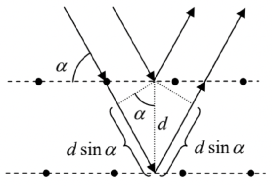 Fig. \(\PageIndex{5}\). The De Broglie wave interference at electron scattering from a crystal lattice.
Thus the founding fathers of quantum mechanics faced a formidable task of reconciling the wave and corpuscular properties of electrons and photons - and other particles. The decisive breakthrough in that task has been achieved in 1926 by Ervin Schrödinger and Max Born, who formulated what is now known either formally as the Schrödinger picture of non-relativistic quantum mechanics of the orbital motion \(^{21}\) in the coordinate representation (this term will be explained later in the course), or informally just as the wave mechanics. I will now formulate the main postulates of this theory.
\({ }^{1}\) See, for example, D. Griffith, Quantum Mechanics, \(2^{\text {nd }}\) ed., Cambridge U. Press, \(2016 .\)
\({ }^{2}\) This famous expression was used in a 1900 talk by Lord Kelvin (born William Thomson), in reference to the results of blackbody radiation measurements and the Michelson-Morley experiments, i.e. the precursors of quantum mechanics and relativity theory.
\({ }^{3}\) See, e.g., EM Sec. 7.8, in particular Eq. (7.211).
\({ }^{4}\) See, e.g., SM Sec. 2.2.
\({ }^{5}\) In the SI units, used throughout this series, \(k_{\mathrm{B}} \approx 1.38 \times 10^{-23} \mathrm{~J} / \mathrm{K}-\) see Appendix CA: Selected Physical Constants for the exact value.
\({ }^{6}\) Max Planck himself wrote \(\hbar \omega\) as \(h v\), where \(v=\omega / 2 \pi\) is the "cyclic" frequency (the number of periods per second) so that in early texts on quantum mechanics the term "Planck’s constant" referred to \(h \equiv 2 \pi \hbar\), while \(\hbar\) was called "the Dirac constant" for a while. I will use the contemporary terminology, and abstain from using the "old Planck’s constant" \(h\) at all, to avoid confusion.
\({ }^{7}\) As a reminder, A. Einstein received his only Nobel Prize (in 1921) for exactly this work, rather than for his relativity theory, i.e. essentially for jumpstarting the same quantum theory which he later questioned.
\({ }^{8}\) For most metals, \(U_{0}\) is between 4 and 5 electron-volts \((\mathrm{eV})\), so that the threshold corresponds to \(\lambda_{\max }=2 \pi c / \omega_{\min }\) \(=2 \pi c /\left(U_{0} / \hbar\right) \approx 300 \mathrm{~nm}\) - approximately at the border between the visible light and the ultraviolet radiation.
\({ }^{9}\) See, e.g., SM Sec. 2.5.
\({ }^{10}\) See, e.g., EM Sec. 8.2.
\({ }^{11}\) The non-relativistic approach to the problem may be justified a posteriori by the fact the resulting energy scale \(E_{\mathrm{H}}\), given by Eq. (\(\PageIndex{14}\)), is much smaller than the electron’s rest energy, \(m_{\mathrm{e}} c^{2} \approx 0.5 \mathrm{MeV}\).
\({ }^{12}\) Unfortunately, another name, the "Rydberg constant", is sometimes used for either this energy unit or its half, \(E_{\mathrm{H}} / 2 \approx 13.6 \mathrm{eV}\). To add to the confusion, the same term "Rydberg constant" is used in some sub-fields of physics for the reciprocal free-space wavelength \(\left(1 / \lambda_{0}=\omega_{0} / 2 \pi c\right)\) corresponding to the frequency \(\omega_{0}=E_{\mathrm{H}} / 2 \hbar\).
\({ }^{13}\) This fact was first noticed and discussed in 1924 by Louis Victor Pierre Raymond de Broglie (in his PhD thesis!), so that instead of speaking of wavefunctions, we are still frequently speaking of the de Broglie waves, especially when free particles are discussed.
\({ }^{14}\) This effect was observed in 1922 , and explained a year later by Arthur Holly Compton, using Eqs. (5) and (15). \({ }^{15}\) See, e.g., EM Sec. 7.1.
\({ }^{16}\) See, e.g., EM Sec. 9.3, in particular Eq. (9.78).
\({ }^{17}\) The constant \(\lambda_{\mathrm{C}}\) that participates in this relation, is close to \(2.46 \times 10^{-12} \mathrm{~m}\), and is called the electron’s Compton wavelength. This term is somewhat misleading: as the reader can see from Eqs. (17)-(19), no wave in the Compton problem has such a wavelength - either before or after the scattering.
\({ }^{18}\) See, e.g., EM Sec. 8.4, in particular Fig. \(8.4.9\) and Eq. (8.82). Frequently, Eq. (\(\PageIndex{22}\)) is called the Bragg condition, due to the pioneering experiments by W. Bragg on X-ray scattering from crystals, which were started in \(1912 .\)
\({ }^{19}\) Later, spectacular experiments on diffraction and interference of heavier particles (with the correspondingly smaller de Broglie wavelength), e.g., neutrons and even \(\mathrm{C}_{60}\) molecules, have also been performed - see, e.g., the review by A. Zeilinger et al., Rev. Mod. Phys. 60, 1067 (1988) and a later publication by O. Nairz et al., Am. J. Phys. 71, 319 (2003). Nowadays, such interference of heavy particles is used, for example, for ultrasensitive measurements of gravity - see, e.g., a popular review by M. Arndt, Phys. Today \(\mathbf{6 7 , 3 0}\) (May 2014), and more recent experiments by S. Abend et al., Phys. Rev. Lett. 117, 203003 (2016).