1.6: Time Evolution

For the time-dependent factor, \(a_{n}(t)\), of each component (57) of the general solution (69), our procedure gave a very simple and universal result (62), describing a linear change of the phase \(\varphi_{n} \equiv\) \(\arg \left(a_{n}\right)\) of this complex function in time, with the constant rate \[\frac{d \varphi_{n}}{d t}=-\omega_{n}=-\frac{E_{n}}{\hbar},\] so that the real and imaginary parts of \(a_{n}\) oscillate sinusoidally with this frequency. The relation (70) coincides with Einstein’s conjecture (5), but could these oscillations of the wavefunctions represent a physical reality? Indeed, for photons, described by Eq. (5), \(E\) may be (and as we will see in Chapter 9 , is) the actual, well-defined energy of one photon, and \(\omega\) is the frequency of the radiation so quantized. However, for non-relativistic particles, described by wave mechanics, the potential energy \(U\), and hence the full energy \(E\), are defined to an arbitrary constant, because we may measure them from an arbitrary reference level. How can such a change of the energy reference level (which may be made just in our mind) alter the frequency of oscillations of a variable?

According to Eqs. (22)-(23), this time evolution of a wavefunction does not affect the particle’s probability distribution, or even any observable (including the energy \(E\), provided that it is always referred to the same origin as \(U\) ), in any stationary state. However, let us combine Eq. (5) with Bohr’s assumption (7): \[\hbar \omega_{n n^{\prime}}=E_{n^{\prime}}-E_{n} .\] The difference \(\omega_{n n}\) ’ of the eigenfrequencies \(\omega_{n}\) and \(\omega_{n}\), participating in this formula, is evidently independent of the energy reference, and as will be proved later in the course, determines the measurable frequency of the electromagnetic radiation (or possibly of a wave of a different physical nature) emitted or absorbed at the quantum transition between the states.

As another but related example, consider two similar particles 1 and 2 , each in the same (say, the lowest-energy) eigenstate, but with their potential energies (and hence the ground state energies \(E_{1,2}\) ) different by a constant \(\Delta U \equiv U_{1}-U_{2}\). Then, according to Eq. (70), the difference \(\varphi \equiv \varphi_{1}-\varphi_{2}\) of their wavefunction phases evolves in time with the reference-independent rate \[\frac{d \varphi}{d t}=-\frac{\Delta U}{\hbar} .\] Certain measurement instruments, weakly coupled to the particles, may allow observation of this evolution, while keeping the particle’s quantum dynamics virtually unperturbed, i.e. Eq. (70) intact. Perhaps the most dramatic measurement of this type is possible using the Josephson effect in weak links between two superconductors \(-\) see Fig. \(7.47\)

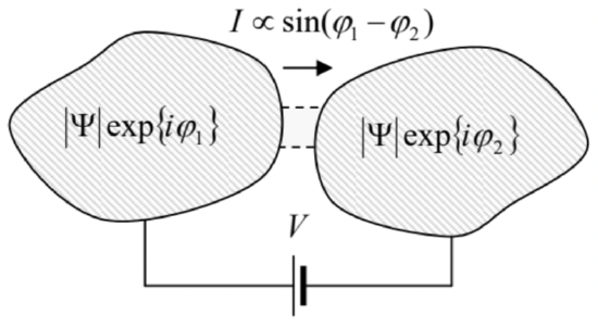Fig. 1.7. The Josephson effect in a weak link between two bulk superconductor electrodes.

As a brief reminder, \({ }^{48}\) superconductivity may be explained by a specific coupling between conduction electrons in solids, that leads, at low temperatures, to the formation of the so-called Cooper pairs. Such pairs, each consisting of two electrons with opposite spins and momenta, behave as Bose particles and form a coherent Bose-Einstein condensate. \({ }^{49}\) Most properties of such a condensate may be described by a single, common wavefunction \(\Psi\), evolving in time just as that of a free particle, with the effective potential energy \(U=q \phi=-2 e \phi\), where \(\phi\) is the electrochemical potential, \({ }^{50}\) and \(q=-2 e\) is the electric charge of a Cooper pair. As a result, for the system shown in Fig. 7, in which externally applied voltage \(V\) fixes the difference \(\phi_{1}-\phi_{2}\) between the electrochemical potentials of two superconductors, Eq. (72) takes the form \[\frac{d \varphi}{d t}=\frac{2 e}{\hbar} V .\] If the link between the superconductors is weak enough, the electric current \(I\) of the Cooper pairs (called the supercurrent) through the link may be approximately described by the following simple relation, \[I=I_{\mathrm{c}} \sin \varphi,\] where \(I_{\mathrm{c}}\) is some constant, dependent on the weak link’s strength. \({ }^{51}\) Now combining Eqs. (73) and (74), we see that if the applied voltage \(V\) is constant in time, the current oscillates sinusoidally, with the socalled Josephson frequency \[\omega_{\mathrm{J}} \equiv \frac{2 e}{\hbar} V,\] as high as \(\sim 484 \mathrm{MHz}\) per microvolt of applied dc voltage. This effect may be readily observed experimentally: though its direct detection is a bit tricky, it is easy to observe the phase locking (synchronization) \(5^{52}\) of the Josephson oscillations by an external microwave signal of frequency \(\omega\). Such phase locking results in the relation \(\omega_{\mathrm{J}}=n \omega\) fulfilled within certain dc current intervals, and hence in the formation, on the weak link’s dc \(I-V\) curve, of virtually vertical current steps at dc voltages \[V_{n}=n \frac{\hbar \omega}{2 e},\] where \(n\) is an integer. \({ }^{53}\) Since frequencies may be stabilized and measured with very high precision, this effect is being used in highly accurate standards of dc voltage.

---

\({ }^{47}\) The effect was predicted in 1962 by Brian Josephson (then a graduate student!) and observed soon after that.

\({ }^{48}\) For a more detailed discussion, including the derivation of Eq. (75), see e.g. EM Chapter 6 .

\({ }^{49}\) A detailed discussion of the Bose-Einstein condensation may be found, e.g., in SM Sec. 3.4.

\({ }^{50}\) For more on this notion see, e.g. SM Sec. 6.3.

\({ }^{51}\) In some cases, the function \(I(\varphi)\) may somewhat deviate from Eq. (74), but these deviations do not affect its fundamental \(2 \pi\)-periodicity, and hence the fundamental relations \((75)-(76)\). (No corrections to them have been found yet.)

\({ }^{52}\) For the discussion of this very general effect, see, e.g., CM Sec. 5.4.

\({ }^{53}\) The size of these dc current steps may be readily calculated from Eqs. (73) and (74). Let me leave this task for the reader’s exercise.