1.8: Dimensionality Reduction

To conclude this introductory chapter, let me discuss the conditions when the spatial dimensionality of a wave-mechanical problem may be reduced. \({ }^{60}\) Naively, one may think that if the particle’s potential energy depends on just one spatial coordinate, say \(U=U(x, t)\), then its wavefunction has to be one-dimensional as well: \(\psi=\psi(x, t)\). Our discussion of the particular case \(U=\) const in the previous section shows that this assumption is wrong. Indeed, though this potential \({ }^{61}\) is just a special case of the potential \(U(x, t)\), most of its eigenfunctions, given by Eqs. (87) or (88), do depend on the other two coordinates. This is why the solutions \(\psi(x, t)\) of the 1D Schrödinger equation \[i \hbar \frac{\partial \Psi}{\partial t}=-\frac{\hbar^{2}}{2 m} \frac{\partial^{2}}{\partial x^{2}} \Psi+U(x, t) \Psi,\] which follows from Eq. (65) by assuming \(\partial \Psi / \partial y=\partial \Psi / \partial z=0\), are insufficient to form the general solution of Eq. (65) for this case.

This fact is easy to understand physically for the simplest case of a stationary 1D potential: \(U=\) \(U(x)\). The absence of the \(y\) - and \(z\)-dependence of the potential energy \(U\) may be interpreted as a potential well that is flat in two directions, \(y\) and \(z\). Repeating the arguments of the previous section for this case, we see that the eigenfunctions of a particle in such a well have the form \[\psi(\mathbf{r})=X(x) \exp \left\{i\left(k_{y} y+k_{z} z\right)\right\},\] where \(X(x)\) is an eigenfunction of the following stationary 1D Schrödinger equation: \[-\frac{\hbar^{2}}{2 m} \frac{d^{2} X}{d x^{2}}+U_{\text {ef }}(x) X=E X,\] where \(U_{\mathrm{ef}}(x)\) is not the full potential energy of the particle, as it would follow from Eq. (92), but rather its effective value including the kinetic energy of the lateral motion: \[U_{\mathrm{ef}} \equiv U+\left(E_{y}+E_{z}\right)=U+\frac{\hbar^{2}}{2 m}\left(k_{y}^{2}+k_{z}^{2}\right) .\] In plain English, the particle’s partial wavefunction \(X(x)\) and its full energy, depend on its transverse momenta, which have continuous spectrum - see the discussion of Eq. (89). This means that Eq. (92) is adequate only if the condition \(k_{y}=k_{z}=0\) is somehow enforced, and in most physical problems, it is not. For example, if a de Broglie (or any other) plane wave \(\Psi(x, t)\) is incident on a potential step, it would be reflected exactly back, i.e. with \(k_{y}=k_{z}=0\), only if the wall’s surface is perfectly plane and exactly normal to the axis \(x\). Any imperfection (and they are so many of them in real physical systems \(-:\) ) may cause excitation of waves with non-zero values of \(k_{y}\) and \(k_{z}\), due to the continuous character of the functions \(E_{y}\left(k_{y}\right)\) and \(E_{z}\left(k_{z}\right){ }^{62}\)

There is essentially one, perhaps counter-intuitive way to make the 1D solutions "robust" to small perturbations: it is to provide a rigid lateral confinement 6 in two other directions. As the simplest example, consider a narrow quantum wire (Fig. 9a), described by the following potential: \[U(\mathbf{r})= \begin{cases}U(x), & \text { for } 0<y<a_{y}, \text { and } 0<z<a_{z}, \\ +\infty, & \text { otherwize. }\end{cases}\]

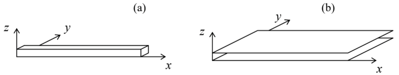Fig. 1.9. Partial confinement in: (a) two dimensions, and (b) one dimension.

Performing the standard variable separation (79), we see that the corresponding stationary Schrödinger equation is satisfied if the partial wavefunction \(X(x)\) obeys Eqs. (94)-(95), but now with a discrete energy spectrum in the transverse directions: \[U_{\text {ef }}=U+\frac{\pi^{2} \hbar^{2}}{2 m}\left(\frac{n_{y}^{2}}{a_{y}^{2}}+\frac{n_{z}^{2}}{a_{z}^{2}}\right) .\] If the lateral confinement is tight, \(a_{y}, a_{z} \rightarrow 0\), then there is a large energy gap, \[\Delta U \sim \frac{\pi^{2} \hbar^{2}}{2 m a_{y, z}^{2}},\] between the ground-state energy of the lateral motion (with \(n_{y}=n_{z}=1\) ) and that for all its excited states. As a result, if the particle is initially placed into the lateral ground state, and its energy \(E\) is much smaller than \(\Delta U\), it would stay in such state, i.e. may be described by a \(1 \mathrm{D}\) Schrödinger equation similar to Eq. (92) - even in the time-dependent case, if the characteristic frequency of energy variations is much smaller than \(\Delta U / \hbar\). Absolutely similarly, the strong lateral confinement in just one dimension (say, \(z\), see Fig. \(9 \mathrm{~b}\) ) enables systems with a robust \(2 \mathrm{D}\) evolution of the particle’s wavefunction.

The tight lateral confinement may ensure the dimensionality reduction even if the potential well is not exactly rectangular in the lateral direction(s), as described by Eq. (96), but is described by some \(x\) and \(t\)-independent profile, if it still provides a sufficiently large energy gap \(\Delta U\). For example, many 2D quantum phenomena, such as the quantum Hall effect, \({ }^{64}\) have been studied experimentally using electrons confined at semiconductor heterojunctions (e.g., epitaxial interfaces \(\mathrm{GaAs} / \mathrm{Al}_{x} \mathrm{Ga}_{1-x} \mathrm{As}\) ), where the potential well in the direction perpendicular to the interface has a nearly triangular shape, and provides an energy gap \(\Delta U\) of the order of \(10^{-2} \mathrm{eV} .{ }^{65}\) This gap corresponds to \(k_{\mathrm{B}} T\) with \(T \sim 100 \mathrm{~K}\), so that careful experimentation at liquid helium temperatures (4K and below) may keep the electrons performing purely 2D motion in the "lowest subband" \(\left(n_{z}=1\right)\).

Finally, note that in systems with reduced dimensionality, Eq. (90) for the number of states at large \(\mathbf{k}\) (i.e., for an essentially free particle motion) should be replaced accordingly: in a \(2 \mathrm{D}\) system of area \(A \gg 1 / k^{2}\), \[d N=\frac{A}{(2 \pi)^{2}} d^{2} k,\] while in a \(1 \mathrm{D}\) system of length \(l \gg 1 / k\), \[d N=\frac{l}{2 \pi} d k,\] with the corresponding changes of the summation rule (91). This change has important implications for the density of states on the energy scale, \(d N / d E\) : it is straightforward (and hence left for the reader :-) to use Eqs. (90), (99), and (100) to show that for free 3D particles the density increases with \(E\) (proportionally to \(E^{1 / 2}\) ), for free \(2 \mathrm{D}\) particles it does not depend on energy at all, while for free \(1 \mathrm{D}\) particles it scales as \(E^{-1 / 2}\), i.e. decreases with energy.

---

\({ }_{60}\) Most textbooks on quantum mechanics jump to the formal solution of 1D problems without such discussion, ignoring the fact that such dimensionality restriction is adequate only under very specific conditions.

\({ }^{61}\) Following tradition, I will frequently use this shorthand for "potential energy", returning to the full term in cases where there is any chance of confusion of this notion with another (say, electrostatic) potential.

\({ }^{62}\) This problem is not specific to quantum mechanics. The classical motion of a particle in a 1D potential may be also unstable with respect to lateral perturbations, especially if the potential is time-dependent, i.e. capable of exciting low-energy lateral modes.

\({ }^{63}\) The term "quantum confinement", sometimes used to describe this phenomenon, is as unfortunate as the "quantum well" term discussed above, because of the same reason: the confinement is a purely classical effect, and as we will repeatedly see in this course, the quantum-mechanical effects reduce, rather than enable it.

\({ }^{64}\) To be discussed in Sec. 3.2.

\({ }^{65}\) See, e.g., P. Harrison, Quantum Wells, Wires, and Dots, \(3^{\text {rd }}\) ed., Wiley, \(2010 .\)

\({ }^{66}\) See, e.g., EM Sec. 8.2.