
10.2: QND Measurements


- Last updated
- Jan 29, 2022
- Save as PDF

( \newcommand{\kernel}{\mathrm{null}\,}\)
I hope that the above discussion has sufficiently illuminated the issues of the group (i), so let me proceed to the question group (ii), in particular to the general issue of the back action of the instrument upon the system under measurement - symbolized with the back arrow in Fig. 1. In the instruments like the Geiger counter, such back action is large: the instrument essentially destroys ("demolishes") the state of the system under measurement. Even the "cleaner" potential-inversion measurement, shown in Fig. 2, fully destroys the initial coherence of the system, i.e. perturbs it rather substantially.
However, in the 1970s it was understood that this is not really necessary. For example, in Sec. 7.3, we have already discussed an example of a two-level system coupled with its environment and described by the Hamiltonian (7.68)-(7.70): ˆH=ˆHs+ˆHint +ˆHe{λ}, with ˆHs=czˆσz, and ˆHint =−f{λ}ˆσz, so that [ˆHs,ˆHint]=0 Comparing this equality with Eq. (4.199), applied to the explicitly-time-independent Hamiltonian ˆHs, iℏ˙ˆHs=[ˆHs,ˆH]≡[ˆHs,(ˆHs+ˆHint+ˆHe{λ})]=[ˆHs,ˆHint]=0, we see that in the Heisenberg picture, the Hamiltonian operator (and hence the energy) of the system of our interest does not change in time. On the other hand, if the "environment" in this discussion is the instrument used for the measurement (see Fig. 1 again), the interaction can change its state, so it may be used to measure the system’s energy - or another observable whose operator commutes with the interaction Hamiltonian. Such a trick is called the quantum non-demolition (QND), or sometimes "backaction-evading" measurements. 10 Due to the lack of back action of the instrument on the corresponding variable, such measurements allow its continuous monitoring. Let me present a fine example of an actual measurement of this kind - see Fig. 3. 11
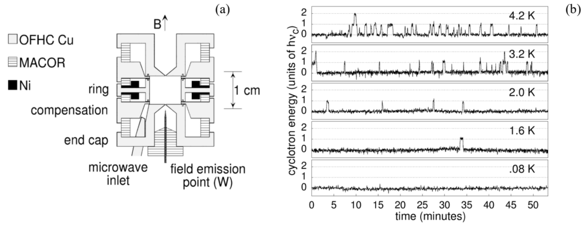
In this experiment, a single electron is captured in a Penning trap - a combination of a (virtually) uniform magnetic field B and a quadrupole electric field. 12 This electric field stabilizes the cyclotron orbits but does not have any noticeable effect on electron motion in the plane perpendicular to the magnetic field, and hence on its Landau level energies - see Eq. (3.50): En=ℏωc(n+12), with ωc=eBme. (In the cited work, with B≈5.3 T, the cyclic frequency ωc/2π was about 147GHz, so that the Landau level splitting ℏωc was close to 10−22 J, i.e. corresponded to kBT at T∼10 K, while the physical temperature of the system might be reduced well below that, down to 80mK ). Now note that the analogy between a Landau-level particle and a harmonic oscillator goes beyond the energy spectrum (14). Indeed, since the Hamiltonian of a 2D particle in a perpendicular magnetic field may be reduced to Eq. (3.47), similar to that of a 1D oscillator, we may repeat all procedures of Sec. 5.4 and rewrite this effective Hamiltonian in the terms of the creation-annihilation operators - see Eq. (5.72): ˆHs=ℏωc(ˆa†ˆa+12). In the Peil and Gabrielse experiment, the trapped electron had one more degree of freedom along the magnetic field. The electric field of the Penning trap created a soft confining potential along this direction (vertical in Fig. 3a; I will take it for the z-axis), so that small electron oscillations along that axis could be well described as those of a 1D harmonic oscillator of much lower eigenfrequency, in that particular experiment with ωz/2π≈64MHz. This frequency could be measured very accurately (with error ∼1 Hz ) by sensitive electronics whose electric field does affect the z-motion of the electron, but not its motion in the perpendicular plane. In an exactly uniform magnetic field, the two modes of electron motion would be completely uncoupled. However, the experimental setup included two special superconducting rings made of niobium (see Fig. 3a), which slightly distorted the magnetic field and created an interaction between the modes, which might be well approximated by the Hamiltonian 13 ˆHint = const ×(ˆa†ˆa+12)ˆz2, so that the main condition (12) of a QND measurement was very closely satisfied. At the same time, the coupling (16) ensured that a change of the Landau level number n by 1 changed the z-oscillation eigenfrequency by ∼12.4 Hz. Since this shift was substantially larger than electronics’ noise, rare spontaneous changes of n (due to a weak uncontrolled coupling of the electron to the environment) could be readily measured - moreover, continuously monitored - see Fig. 3b. The record shows spontaneous excitations of the electron to higher Landau levels, with its sequential relaxation, just as described by Eqs. (7.208)-(7.210). The detailed data statistics analysis showed that there was virtually no effect of the measuring instrument on these processes - at least on the scale of minutes, i.e. as many as ∼1013 cyclotron orbit periods. 14
It is important, however, to note that any measurement - QND or not - cannot avoid the uncertainty relations between incompatible variables; in the particular case described above, continuous monitoring of the Landau state number n does not allow the simultaneous monitoring of its quantum phase (which may be defined exactly as in the harmonic oscillator). In this context, it is natural to wonder whether the QND measurement concept may be extended from quadratic-form variables like energy to "usual" observables such as coordinates and momenta. whose uncertainties are bound by the ordinary Heisenberg’s relation (1.35). The answer is yes, but the required methods are a bit more tricky.
For example, let us place an electrically charged particle into a uniform electric field E=nxE(t) of an instrument, so that their interaction Hamiltonian is
ˆHint =−qˆE(t)ˆx. Such interaction may certainly pass the information on the time evolution of the coordinate x to the instrument. However, in this case, Eq. (12) is not satisfied - at least for the kinetic-energy part of the particle’s Hamiltonian; as a result, the interaction distorts its time evolution. Indeed, writing the Heisenberg equation (4.199) for the x-component of the momentum, we get ˙ˆp−˙ˆp|ε=0=qˆE(t). On the other hand, integrating Eq. (5.139) for the coordinate operator evolution, 15 we get the expression ˆx(t)=ˆx(t0)+1m∫tt0ˆp(t′)dt′, which shows that the perturbations (18) of the momentum eventually find their way to the coordinate evolution, not allowing its unperturbed sequential measurements.
However, for such an important particular system as a harmonic oscillator, the following trick is possible. For this system, Eqs. (5.139) with the addition (18) may be readily combined to give a secondorder differential equation for the coordinate operator, that is absolutely similar to the classical equation of motion of the system, and has a similar solution: 16 ˆx(t)=ˆx(t)|ε=0+qmω0∫t−∞ˆE(t′)sinω0(t−t′)dt′. This formula confirms that generally, the external field E(t) (in our case, the sensing field of the measurement instrument) affects the time evolution law - of course. However, Eq. (20) shows that if the field is applied only at moments t′n separated by intervals π2, where τ≡2π/ω0 is the oscillation period, its effect on coordinate vanishes at similarly spaced observation instants tn=tn++(m+1/2)τ. This is the idea of stroboscopic QND measurements. Of course, according to Eq. (18), even such measurement strongly perturbs the oscillator momentum, so that even if the values xn are measured with high accuracy, the Heisenberg’s uncertainty relation is not violated.A direct implementation of the stroboscopic measurements is technically complicated, but this initial idea has opened a way to more practicable solutions. For example, it is straightforward to use the Heisenberg equations of motion to show that if the coupling of two harmonic oscillators, with coordinates x and X, and unperturbed frequencies ω and Ω, is modulated in time as ˆHint ∝ˆxˆXcosωtcosΩt, then the process in one of the oscillators (say, that with frequency Ω ) does not affect dynamics of one of the quadrature components of the counterpart oscillator, defined by relations 17 ˆx1≡ˆxcosωt−ˆpmωsinωt,ˆx2≡ˆxsinωt+ˆpmωcosωt, while this component’s motion does affect the dynamics of one of the quadrature components of the counterpart oscillator. (For the counterpart couple of quadrature components, the information transfer goes in the opposite direction.) This scheme has been successfully used for QND measurements. 18
Please note that the last two QND measurement examples are based on the idea of a periodic change of a certain parameter in time - either in the short-pulse form or the sinusoidal form. If the only goal of a QND measurement is a sensitive measurement of a weak classical force acting on a quantum probe system, i.e. a 1D oscillator of eigenfrequency ω0, it may be implemented much simpler - just by modulating an oscillator’s parameter with a frequency ω≈2ω0. From the classical dynamics, we know that if the depth of such modulation exceeds a certain threshold value, it results in the excitation of the so-called degenerate parametric oscillations with frequency ω/2≈ω0, and one of two opposite phases. 19 In the language of Eq. (22), the parametric excitation means exponential growth of one of the quadrature components (with its sign depending on initial conditions), while the counterpart component is suppressed. Close to, but below the excitation threshold, the parameter modulation boosts all fluctuations of the almost-excited component, including its quantum-mechanical uncertainty, and suppresses (squeezes) those of the counterpart component. The result is a squeezed state, already discussed in Sec. 5.5 of this course (see in particular Eqs. (5.143) and Fig. 5.8), which allows one to notice the effect of an external force on the oscillator on the backdrop of a quantum uncertainty much smaller than the standard quantum limit (5.99).
In electrical engineering, this fact may be conveniently formulated in terms of noise parameter ΘN of a linear amplifier - essentially the tool for continuous monitoring of an input "signal" - e.g., a microwave or optical waveform. 20 Namely, ΘN of "usual" (say, transistor or maser) amplifiers which are equally sensitive to both quadrature components of the signal, ΘN has the minimum value ℏω/2, due to the quantum uncertainty pertinent to the quantum state of the amplifier itself (which therefore plays the role of its "quantum noise") - the fact that was recognized in the early 1960 s.21 On the other hand, a degenerate parametric amplifier, sensitive to just one quadrature component, may have ΘN well below ℏω/2, due to its ground state squeezing. 22
Let me note that the parameter-modulation schemes of the QND measurements are not limited to harmonic oscillators, and may be applied to other important quantum systems, notably including twolevel (i.e. spin- 1/2-like) systems. 23 Such measurements may be an important tool for the further progress of quantum computation and cryptography. 24
Finally, let me mention that the composite systems consisting of a quantum subsystem, and a classical subsystem performing its continuous weakly-perturbing measurement and using its results for providing a specially crafted feedback to the quantum subsystem, may have some curious properties, in particular mock a quantum system detached from the environment. 25
10 For a detailed discussion of this field see, e.g., V. Braginsky and F. Khalili (ed. by K. Thorne), Quantum Measurement, Cambridge U. Press, 1992; for an earlier review, see V. Braginsky et al., Science 209, 547 (1980).
11 S. Peil and G. Gabrielse, Phys. Rev. Lett. 83, 1287 (1999).
12 It is similar to the 2D system discussed in EM Sec. 2.7, but with additional rotation about one of the axes.
13 Here I have simplified the real situation a bit. Actually, in that experiment, there was an electron spin’s contribution to the interaction Hamiltonian as well, but since the used high magnetic field polarized the spins quite reliably, their only effect was a constant shift of the frequency ωz, which is not important for our discussion.
14 See also the conceptually similar experiments, performed by different means: G. Nogues et al., Nature 400,239 (1999).
15 This simple relation is limited to 1D systems with Hamiltonians of the type (1.41), but by now the reader certainly knows enough to understand that this discussion may be readily generalized to many other systems.
16 Note in particular that the function sinω0τ (with τ≡t−t′ ) under the integral, divided by ω0, is nothing more than the temporal Green’s function G(τ) of a loss-free harmonic oscillator - see, e.g., CM Sec. 5.1.
17 The physical sense of these relations should be clear from Fig. 5.8: they define a system of coordinates rotating clockwise with the angular velocity equal to ω, so that the point representing unperturbed classical oscillations with that frequency is at rest in this rotating frame. (The "probability cloud" representing a Glauber state is also stationary in the coordinates [x1,x2].) The reader familiar with the classical theory oscillations may notice that the observables x1 and x2 so defined are just the Poincaré plane coordinates ("RWA variables") - see, e.g., CM Sec. 5.3-5.6, and especially Fig. 5.9, where these coordinates are denoted as u and v.
18 The first, initially imperfect QND experiments were reported by R. Slusher et al., Phys. Rev. Lett. 55,2409 (1985), and other groups soon after this, using nonlinear interactions of optical waves. Later, the results were much improved - see, e.g., P. Grangier et al., Nature 396, 537 (1998), and references therein. Recently, such experiments were extended to mechanical systems - see, e.g., F. Lecocq et al., Phys. Rev. X5,041037 (2015).
19 See, e.g., CM Sec. 5.5, and also Fig. 5.8 and its discussion in Sec. 5.6.
20 For a quantitative definition of the latter parameter, suitable for the quantum sensitivity range (ΘN∼ℏω) as well, see, e.g., I. Devyatov et al., J. Appl. Phys. 60, 1808 (1986). In the classical noise limit (ΘN≫λω), it coincides with kBTN, where TN is a more popular measure of electronics’ noise, called the noise temperature.
21 See, e.g., H. Haus and J. Mullen, Phys. Rev. 128, 2407 (1962).
22 See, e.g., the spectacular experiments by B. Yurke et al., Phys. Rev. Lett. 60,764 (1988). Note also that the squeezed ground states of light are now used to improve the sensitivity of interferometers in gravitational wave detectors - see, e.g., the recent review by R. Schnabel, Phys. Repts. 684,1 (2017), and the later paper by F. Acernese et al., Phys. Rev. Lett. 123, 231108 (2019).
23 See, e.g., D. Averin, Phys. Rev. Lett. 88, 207901 (2002).
24 See, e.g., G. Jaeger, Quantum Information: An Overview, Springer, 2006.
25 See, e.g., the monograph by H. Wiseman and G. Milburn, Quantum Measurement and Control, Cambridge U. Press (2009), more recent experiments by R. Vijay et al., Nature 490,77 (2012), and references therein.