2: Basic concepts of quantum mechanics
- Page ID
- 50554
\( \newcommand{\vecs}[1]{\overset { \scriptstyle \rightharpoonup} {\mathbf{#1}} } \)
\( \newcommand{\vecd}[1]{\overset{-\!-\!\rightharpoonup}{\vphantom{a}\smash {#1}}} \)
\( \newcommand{\id}{\mathrm{id}}\) \( \newcommand{\Span}{\mathrm{span}}\)
( \newcommand{\kernel}{\mathrm{null}\,}\) \( \newcommand{\range}{\mathrm{range}\,}\)
\( \newcommand{\RealPart}{\mathrm{Re}}\) \( \newcommand{\ImaginaryPart}{\mathrm{Im}}\)
\( \newcommand{\Argument}{\mathrm{Arg}}\) \( \newcommand{\norm}[1]{\| #1 \|}\)
\( \newcommand{\inner}[2]{\langle #1, #2 \rangle}\)
\( \newcommand{\Span}{\mathrm{span}}\)
\( \newcommand{\id}{\mathrm{id}}\)
\( \newcommand{\Span}{\mathrm{span}}\)
\( \newcommand{\kernel}{\mathrm{null}\,}\)
\( \newcommand{\range}{\mathrm{range}\,}\)
\( \newcommand{\RealPart}{\mathrm{Re}}\)
\( \newcommand{\ImaginaryPart}{\mathrm{Im}}\)
\( \newcommand{\Argument}{\mathrm{Arg}}\)
\( \newcommand{\norm}[1]{\| #1 \|}\)
\( \newcommand{\inner}[2]{\langle #1, #2 \rangle}\)
\( \newcommand{\Span}{\mathrm{span}}\) \( \newcommand{\AA}{\unicode[.8,0]{x212B}}\)
\( \newcommand{\vectorA}[1]{\vec{#1}} % arrow\)
\( \newcommand{\vectorAt}[1]{\vec{\text{#1}}} % arrow\)
\( \newcommand{\vectorB}[1]{\overset { \scriptstyle \rightharpoonup} {\mathbf{#1}} } \)
\( \newcommand{\vectorC}[1]{\textbf{#1}} \)
\( \newcommand{\vectorD}[1]{\overrightarrow{#1}} \)
\( \newcommand{\vectorDt}[1]{\overrightarrow{\text{#1}}} \)
\( \newcommand{\vectE}[1]{\overset{-\!-\!\rightharpoonup}{\vphantom{a}\smash{\mathbf {#1}}}} \)
\( \newcommand{\vecs}[1]{\overset { \scriptstyle \rightharpoonup} {\mathbf{#1}} } \)
\( \newcommand{\vecd}[1]{\overset{-\!-\!\rightharpoonup}{\vphantom{a}\smash {#1}}} \)
\(\newcommand{\avec}{\mathbf a}\) \(\newcommand{\bvec}{\mathbf b}\) \(\newcommand{\cvec}{\mathbf c}\) \(\newcommand{\dvec}{\mathbf d}\) \(\newcommand{\dtil}{\widetilde{\mathbf d}}\) \(\newcommand{\evec}{\mathbf e}\) \(\newcommand{\fvec}{\mathbf f}\) \(\newcommand{\nvec}{\mathbf n}\) \(\newcommand{\pvec}{\mathbf p}\) \(\newcommand{\qvec}{\mathbf q}\) \(\newcommand{\svec}{\mathbf s}\) \(\newcommand{\tvec}{\mathbf t}\) \(\newcommand{\uvec}{\mathbf u}\) \(\newcommand{\vvec}{\mathbf v}\) \(\newcommand{\wvec}{\mathbf w}\) \(\newcommand{\xvec}{\mathbf x}\) \(\newcommand{\yvec}{\mathbf y}\) \(\newcommand{\zvec}{\mathbf z}\) \(\newcommand{\rvec}{\mathbf r}\) \(\newcommand{\mvec}{\mathbf m}\) \(\newcommand{\zerovec}{\mathbf 0}\) \(\newcommand{\onevec}{\mathbf 1}\) \(\newcommand{\real}{\mathbb R}\) \(\newcommand{\twovec}[2]{\left[\begin{array}{r}#1 \\ #2 \end{array}\right]}\) \(\newcommand{\ctwovec}[2]{\left[\begin{array}{c}#1 \\ #2 \end{array}\right]}\) \(\newcommand{\threevec}[3]{\left[\begin{array}{r}#1 \\ #2 \\ #3 \end{array}\right]}\) \(\newcommand{\cthreevec}[3]{\left[\begin{array}{c}#1 \\ #2 \\ #3 \end{array}\right]}\) \(\newcommand{\fourvec}[4]{\left[\begin{array}{r}#1 \\ #2 \\ #3 \\ #4 \end{array}\right]}\) \(\newcommand{\cfourvec}[4]{\left[\begin{array}{c}#1 \\ #2 \\ #3 \\ #4 \end{array}\right]}\) \(\newcommand{\fivevec}[5]{\left[\begin{array}{r}#1 \\ #2 \\ #3 \\ #4 \\ #5 \\ \end{array}\right]}\) \(\newcommand{\cfivevec}[5]{\left[\begin{array}{c}#1 \\ #2 \\ #3 \\ #4 \\ #5 \\ \end{array}\right]}\) \(\newcommand{\mattwo}[4]{\left[\begin{array}{rr}#1 \amp #2 \\ #3 \amp #4 \\ \end{array}\right]}\) \(\newcommand{\laspan}[1]{\text{Span}\{#1\}}\) \(\newcommand{\bcal}{\cal B}\) \(\newcommand{\ccal}{\cal C}\) \(\newcommand{\scal}{\cal S}\) \(\newcommand{\wcal}{\cal W}\) \(\newcommand{\ecal}{\cal E}\) \(\newcommand{\coords}[2]{\left\{#1\right\}_{#2}}\) \(\newcommand{\gray}[1]{\color{gray}{#1}}\) \(\newcommand{\lgray}[1]{\color{lightgray}{#1}}\) \(\newcommand{\rank}{\operatorname{rank}}\) \(\newcommand{\row}{\text{Row}}\) \(\newcommand{\col}{\text{Col}}\) \(\renewcommand{\row}{\text{Row}}\) \(\newcommand{\nul}{\text{Nul}}\) \(\newcommand{\var}{\text{Var}}\) \(\newcommand{\corr}{\text{corr}}\) \(\newcommand{\len}[1]{\left|#1\right|}\) \(\newcommand{\bbar}{\overline{\bvec}}\) \(\newcommand{\bhat}{\widehat{\bvec}}\) \(\newcommand{\bperp}{\bvec^\perp}\) \(\newcommand{\xhat}{\widehat{\xvec}}\) \(\newcommand{\vhat}{\widehat{\vvec}}\) \(\newcommand{\uhat}{\widehat{\uvec}}\) \(\newcommand{\what}{\widehat{\wvec}}\) \(\newcommand{\Sighat}{\widehat{\Sigma}}\) \(\newcommand{\lt}{<}\) \(\newcommand{\gt}{>}\) \(\newcommand{\amp}{&}\) \(\definecolor{fillinmathshade}{gray}{0.9}\)In this chapter we introduce the Schrödinger equation, the dynamic equation describing a quantummechanical system. We discuss the role of energy eigenvalues and eigenfunctions in the process of finding it’s solutions. Through the problem of linear harmonic oscillator the way one solves quantum mechanical problems is demonstrated. Finally the expectation value and the variance of an operator is discussed.
Elements of differential equations, and the material of Chapter 1. The classical equations of motions. The classical harmonic oscillator.
The Schrödinger equation
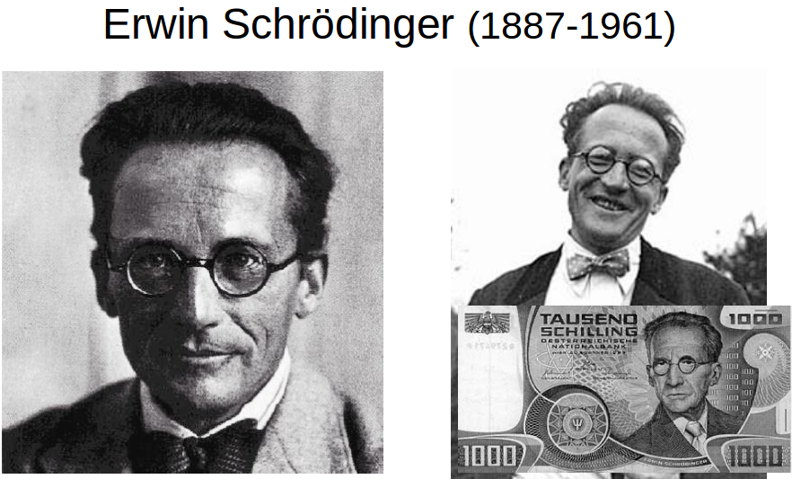
As we have seen in the previous section, the state of a particle in position space is described by a wave function \(\Psi(x, t)\) in one, or \(\Psi(\mathbf{r}, t)\) in three dimensions. This is a probability amplitude, and \(\left.\Psi(\mathbf{r}, t)\right|^{2}\) is the probability density of finding the particle somewhere in space around the position given by the vector r. It was Erwin Schrödinger who wrote up the equation, the solutions of which gives us the concrete form of the function. His fundamental equation is called the time dependent Schrödinger equation, or dynamical equation, and has the form:
\(i \hbar \frac{\partial \Psi(\mathbf{r}, t)}{\partial t}=-\frac{\hbar^{2}}{2 m} \Delta \Psi(\mathbf{r}, t)+V(\mathbf{r}) \Psi(\mathbf{r}, t)\) (2.1)
To simplify the treatment we consider in this subsection the one dimensional motion along the x axis:
\(i \hbar \frac{\partial \Psi(x, t)}{\partial t}=-\frac{\hbar^{2}}{2 m} \frac{\partial^{2} \Psi(x, t)}{\partial x^{2}}+V(x) \Psi(x, t)\) (2.2)
In quantum mechanics the right hand side of the Schrödinger equation is written shortly as \(\hat{H} \Psi(x, t)\), so (2.2) can be written as
\(i \hbar \frac{\partial \Psi(x, t)}{\partial t}=\hat{H} \Psi(x, t)\) (2.3)
This notation has a deeper reason, which is explained here shortly. The operation \(-\frac{\hbar^{2}}{2 m} \frac{\partial^{2} \Psi(x, t)}{\partial x^{2}}+V(x) \Psi(x, t)\) can be considered as a transformation of the function \(\Psi(x, t)\), and the result is a another function of x and t. This means that the right hand side is a (specific) mapping from the set of functions to give again a function. The mapping is linear, and
\(\hat{H}=-\frac{\hbar^{2}}{2 m} \frac{\partial^{2}}{\partial x^{2}}+V(x)\) (2.4)
is a linear transformation or linear operator, as it is called in quantum mechanics. The operator in question \(\hat{H}\) is called the operator of the energy, that bears the name the Hamilton operator or the Hamiltonian for short. Later on, besides \(\hat{H}\) we shall encounter other types of linear operators, corresponding to physical quantities other than the energy. The form (2.4) of the Hamiltonian is used for the specific problem of a particle moving in one dimension x, where the external force field given by the potential energy function \(V(x)\). For other problems the expression of the Hamiltonian is different, but the dynamical equation in the form (2.3) is the same. This is like in classical mechanics where the equation of motion for one particle is always \(\dot{\mathbf{p}}=\mathbf{F}\) but \(\mathbf{F}\), the force depends on the physical situation in question. In quantum mechanics the Schrödinger equation replaces Newton’s equation of motion of classical mechanics which shows its fundamental significance.
We enumerate here a few important properties of the equation (2.2), or equivalently those of eq. (2.3):
- It is a linear equation, which means that if \(\Psi_{1}(x, t)\) and \(\Psi_{2}(x, t)\) are solutions of the equation, then linear combinations of the form \(c_{1} \Psi_{1}+c_{2} \Psi_{2}\) will be also a solution, where \(c_{1}\) and \(c_{2}\) are complex constants. The summation can be extended to infinite sums, (with certain mathematical restrictions). Linearity is valid, because on both sides of the equation we have linear operations, derivations and multiplication with the given function \(V(x)\).
- Another important property is that the equation is of first order in time. Therefore if we give an initial function at \(t = t_{0}\) depending only on x: \(\Psi\left(x, t_{0}\right) \equiv \psi_{0}(x)\), then by solving the equation we can find – in principle – a unique solution that satisfies this initial condition. There are of course infinitely many possible solutions, but they correspond to different initial conditions. The time dependence of the wave function from a given initial condition is called time evolution.
- The equation conserves the norm of the wave function, which means that if \(\Psi(x, t)\) obeys (2.2), then the integral of the position probability density with respect to x is constant independently of t. Specifically, if this integral is equal to 1 at t0, then it remains so for all times.
\(\int_{-\infty}^{\infty}\left|\psi_{0}(x)\right|^{2} d x=1 \Longrightarrow \int_{-\infty}^{\infty}|\Psi(x, t)|^{2} d x=1, \quad \forall t\) (2.5)
In other words the normalization property remains valid for all times. This property is called unitarity of the time evolution. The proof of this statement is left as a problem.
Using (2.2) prove that the time derivative of the normalization condition is zero, which means the validity of (2.5).
Stationary states
Specific solutions of eq. (2.2) can be found by making the "ansatz" (this German word used also in English math texts, and means educated guess), that the solution is a product of two functions
\(\Psi(x, t)=a u(t) u(x)\) (2.6)
where \(au(t)\) depends only on time, while \(u(x)\) is a space dependent function. This procedure is called separation. Not all the solutions of Eq. (2.2) have this separated form, but it is useful to find first these kind of solutions. Substituting back the product (2.6) into (2.2), we find
\(i \hbar u(x) \frac{\partial a u(t)}{\partial t}=\left(-\frac{\hbar^{2}}{2 m} \frac{\partial^{2} u(x)}{\partial x^{2}}+V(x) u(x)\right) a u(t)\) (2.7)
Dividing by \(au(t)u(x)\), we get:
\(i \hbar \frac{1}{a u(t)} \frac{\partial a u(t)}{\partial t}=\frac{1}{u(x)}\left(-\frac{\hbar^{2}}{2 m} \frac{\partial^{2} u(x)}{\partial x^{2}}+V(x) u(x)\right)\) (2.8)
As the function on the left hand side depends only on time, while the one on the right hand side depends only on xx, and they must be equal for all values of these variables, this is possible only if both sides are equal to a constant independent of x and t. It is easy to check that the constant has to be of dimension of energy, and will be denoted by ε. We get then two equations. One of them is
\(i \hbar \frac{\partial a u(t)}{\partial t}=a u(t) \varepsilon\) (2.9)
with the solution
\(a u(t)=C e^{-i \varepsilon t / \hbar}\) (2.10)
where C is an integration constant.
The other equation takes the form:
\(-\frac{\hbar^{2}}{2 m} \frac{\partial^{2} u(x)}{\partial x^{2}}+V(x) u(x)=\varepsilon u(x)\) (2.11)
We recognize that on the left hand side we have now again the operator \(\hat{H}\) acting this time on \(u(x)\):
\(\hat{H} u(x)=\varepsilon u(x)\) (2.12)
This is a so called eigenvalue problem: the effect of the operator is such that it gives back the function itself multiplied by a constant. As the operator here is the Hamiltonian, i.e. the energy operator, (2.12) is an energy eigenvalue equation. Sometimes it is also called the (time independent) Schrödinger equation, but we shall not use this terminology.
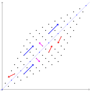
This simple gif animation tries to visualize the concepts of eigenvectors.
http://upload.wikimedia.org/Wikipedia/commons/0/06/Eigenvectors.gif
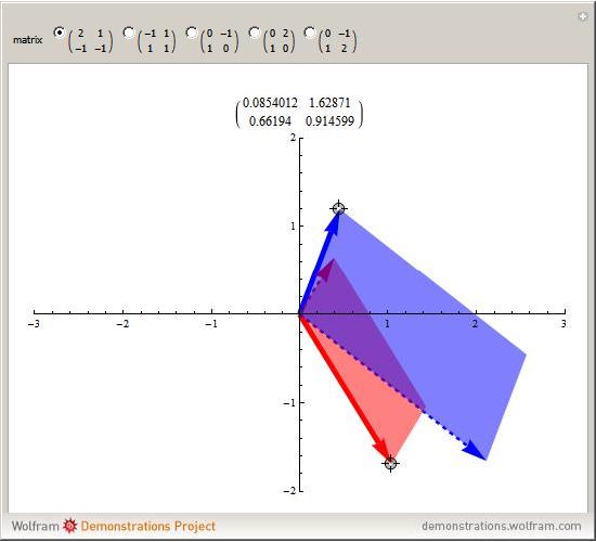
Drag each vector until the coloured parallelogram vanishes. If you can do this for two independent vectors, they form a basis of eigenvectors and the matrix of the linear map becomes diagonal, that is, nondiagonal terms are zero. This is impossible for some of the initial matrices—try them all. When you have found an eigenvector, check that it can be prolonged in its own direction while remaining an eigenvector; it is interesting to keep an eye on the matrix at the same time.
It is important to stress here that Eq. (2.11) must be considered together with certain boundary conditions to be satisfied by the solutions \(u(x)\) at the boundaries of their domain. In other words the boundary conditions are parts of the notion of the differential operator \(\hat{H}\) in (2.11). The boundary conditions can be chosen in several different ways, and in general, physical considerations are used to choose the appropriate ones. In other words among the solutions of (2.11) one has to select those special ones where \(u(x)\) obeys the boundary conditions which is usually possible only for certain specific values of ε. The functions \(u_{ε}(x)\) obeying the equation with the given boundary conditions are called the eigenfunctions of \(\hat{H}\) belonging to the corresponding energy eigenvalue ε: \(\hat{H} u_{\varepsilon}(x)=\varepsilon u_{\varepsilon}(x)\).
According to the separation condition all the functions of the form
\(\psi_{\varepsilon}(x, t)=u_{\varepsilon}(x) e^{-i \varepsilon t / \hbar}\) (2.13)
will be the solutions of the Schrödinger equation (2.2). The allowed energy eigenvalues εε, selected by the boundary conditions can be discrete, then they are usually labeled by integers \(ε_{n}(n=1, 2,⋯)\), but they can also be continuous. In the latter case one finds proper solutions for all ε-s within a certain energy interval. It can be easily shown that the physically acceptable solutions must belong to real energy eigenvalues.
Show that the normalization condition allows only real values of ε.
In general, there are infinitely many solutions of the form (2.13), but they do not exhaust all the solutions. As the Hamiltonian, as well as the Schrödinger-equation are linear, appropriate linear combinations of the specific solutions (2.13) also obey the Schrödinger equation, and have the general form:
\(\Psi(x, t)=\sum_{n} c_{n} u_{n}(x) e^{-i \varepsilon_{n} t / \hbar}+\int c(\varepsilon) u_{\varepsilon}(x) e^{-i \varepsilon t / \hbar} d \varepsilon\) (2.14)
Here the complex numbers cncn and the complex function \(c(ε)\) are arbitrary, the only condition is that the resulting \(Ψ(x,t)\) must be normalizable, i.e. they must be such that the condition \(\int|\Psi(x, t)|^{2} d x=1\) must hold.
It can also be shown – although this is usually far from simple – that for physically adequate potential energy functions, or \(\hat{H}\) operators, all the solutions of (2.2) can be written in the form as given by (2.14).
The solutions \(ψ_{ε}(x,t)\) of the form (2.13) are seen to be specific in the sense that they contain only a single term from the sum or integral in (2.14). Therefore the probability distributions corresponding to these solutions: \(\left|\psi_{\varepsilon}(x, t)\right|^{2}=\left|u_{\varepsilon}(x)\right|^{2}\) do not depend on time, while the wave functions i.e. the probability amplitudes are time dependent. These wave functions, and the corresponding physical states are called stationary states. According to (2.14) a general solution can be obtained by an expansion in terms of the stationary states.
The set of all eigenvalues is called the spectrum of the \(\hat{H}\) operator, or the energy spectrum. Note that this terminology is different from the notion of the spectrum in experimental spectroscopy, but – as we will see – they are related to each other. In experimental spectroscopy an energy eigenvalue is called a term, and the spectrum seen e.g. in optical spectroscopy is the frequency corresponding to energy eigenvalue differences. The energy eigenfunctions belonging to given eigenvalues can be identified with the stationary states (orbits) postulated by Bohr. Therefore the existence of stationary states is the quantum mechanical proof of Bohr’s first postulate. In addition QM also gives us the method how to find the energies and wave functions of the stationary states.
Now we shall introduce the following important property of the eigenfunctions of \(\hat{H}\). It can be proven, that the integral of the product \(u_{n}^{*}(x) u_{n^{\prime}}(x)\) of eigenfunctions belonging to different eigenvalues \(\varepsilon_{n} e q \varepsilon_{n^{\prime}}\) vanishes \(\int u_{n}^{*}(x) u_{n^{\prime}}(x) d x=0\), where the limits of the integration is taken over the domain of the eigenfunctions, usually between \(−∞\) and \(∞\). This property is called orthogonality of the eigenfunctions. If we also prescribe the normalization of the eigenfunctions, which can be always achieved by multiplying with an appropriate constant, we can write
\(\int u_{n}^{*}(x) u_{n^{\prime}}(x) d x=\delta_{n n^{\prime}}\) (2.15)
where \(\delta_{n n^{\prime}}\) is Kronecker’s symbol. Both orthogonality and normalization is taken together here, and we say therefore that the eigenfunctions are orthonormal.
There is a little more complicated but important point here. It may turn out, that one finds several linearly independent solutions of (2.11) with one and the same ε. Let the number of these solutions belonging to ε be \(g_{ε}\). We say that ε is \(g_{ε}\) times degenerate. It can also be proven that among the degenerate solutions there are orthogonal ones whose number is \(g_{ε}\). We can write this in the following way:
\(\int u_{n k}^{*}(x) u_{n k^{\prime}}(x) d x=\delta_{k k^{\prime}}\) (2.16)
where \(u_{nk}(x)\) means the k-th solution belonging to a given \(\varepsilon_{n}: k=1,2 \ldots g_{\varepsilon_{n}}\).
Show that the probability density obtained from the linear combination of two stationary states belonging to different energy eigenvalues depends on time. What is the characteristic time dependence of this probability density?
An example: the linear harmonic oscillator
This is a very important system both in classical and in quantum physics, so besides demonstrating the way one solves quantum mechanical problems, it has far reaching applications in all branches of theoretical physics
The potential energy is \(\frac{1}{2} D x^{2}=\frac{1}{2} m \omega^{2} x^{2}\), and the eigenvalue equation is
\(-\frac{\hbar^{2}}{2 m} \frac{\partial^{2} u}{\partial x^{2}}+\frac{1}{2} m \omega^{2} x^{2} u(x)=\varepsilon u(x)\) (2.17)
where \(−∞<x<∞\)
It will be useful to introduce the dimensionless coordinate ξ and the dimensionless energy ϵ by the relations:
\(\xi=\sqrt{m \omega / \hbar} x, \quad \epsilon=\frac{2 \varepsilon}{\hbar \omega}\) (2.18)
We obtain from (2.17)
\(\frac{\partial^{2} u}{\partial \xi^{2}}+\left(\epsilon-\xi^{2}\right) u=0\) (2.19)
We first find the asymptotic solution of this equation. For large values of \(|\xi|\) we have \(\frac{\partial^{2} u}{\partial \xi^{2}}-\xi^{2} u=0\), with the approximate solution \(e^{-\xi^{2} / 2}\). (The term \(\xi^{2} e^{-\xi^{2} / 2}\) will dominate over \(e^{-\xi^{2} / 2}\) for large \(|\xi|\)) The other possibility \(e^{+\xi^{2} / 2}\) must be omitted, because it is not square integrable, so it is not an allowed function to describe a quantum state.
The exact solutions of (2.19) are to be found in the form
\(u(\xi)=\mathcal{H}(\xi) e^{-\xi^{2} / 2}\) (2.20)
where \(\mathcal{H}(\xi)\) is a polynomial of \(\xi\). Substituting this assumption into 2.19, we get the equation
\(\frac{d^{2} \mathcal{H}}{d \xi^{2}}-2 \xi \frac{d \mathcal{H}}{d \xi}+(\epsilon-1) \mathcal{H}=0\) (2.21)
This is known as the differential equation for the Hermite polynomials. Looking for its solution as a power series \(\mathcal{H}=\sum_{k} a_{k} \xi^{k}\), we find that the coefficients have to obey the recursion condition
\((2 k-\epsilon+1) a_{k}=(k+2)(k+1) a_{k+2}\) (2.22)
Derive (2.21) from the assumption (2.20) and (2.19). Derive the recursion formula, for the coefficients of the power series.
In case the series would be an infinite one, for large k-s we would have \(a_{k+2} \simeq 2 k a_{k}\), which is obtained by keeping only the highest order terms in k on both sides. This recursion relation is, however, the property of the series of \(e^{\xi^{2}}\) which would lead to a non square integrable function as the asymptotic form of u would then be again \(e^{\xi^{2}} e^{-\xi^{2} / 2}=e^{\xi^{2} / 2}\). Therefore the sum determining \(\mathcal{H}\) must remain finite, and so it has to terminate at a certain integer power, we shall denote it by \(\nu\). This means that all the coefficients higher than \(\nu\) are zero, and in particular:
\(a_{\nu} e q 0, \quad a_{\nu+1}=0, \quad a_{\nu+2}=0\) (2.23)
In other words \(\mathcal{H}\) is a polynomial of degree \(\nu\), and the condition \(a_{\nu+1}=0\) requires then that all the coefficients \(0=a_{\nu-1}=a_{\nu-3}=\ldots\) so the polynomials are either even or odd, depending on \(\nu\). In view of 2.23 we get 2.22 that \(2\nu-\epsilon+1=0\), or \(\epsilon=2\nu+1\).
To summarize the result the eigenvalue equation has square integrable solutions only if
\(\varepsilon_{\nu}=\hbar \omega\left(\nu+\frac{1}{2}\right), \quad \nu=0,1,2 \ldots\) (2.24)
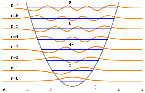
where \(\nu\) is called the vibrational quantum number. The possible energy values of the harmonic oscillator are equidistant with the separation \(Δε=ℏω\). The lowest energy for \(\nu=0\), \(\varepsilon_{0}=\hbar \omega / 2\) is not zero, but equals half of the level separation. ε0 is called zero-point energy.
The corresponding eigenfunctions are
\(u_{\nu}(x)=\mathcal{N}_{\nu} \mathcal{H}_{\nu}\left(\sqrt{\frac{m \omega}{\hbar}} x\right) e^{-\frac{m \omega}{\hbar} x^{2} / 2}\) (2.25)
where \(\mathcal{H}_{\nu}\) -s are polynomials of degree \(\nu\), called Hermite polynomials, and \(\mathcal{N}_{\nu}\)-s are normalization coefficients. The square integrability is ensured by the exponential factor. For the highest nonvanishing coefficient of \(\mathcal{H}_{\nu}\), which is not determined by the recursion, the convention is to set \(a_{\nu}=2^{\nu}\).
Determine the first 3 Hermite polynomials
It can be shown that the \(\epsilon_{\nu}\) eigenvalues are nondegenerate, so the eigenfunction \(u_{\nu}(x)\) is unique (up to a constant factor). The eigenfunctions have also the important property of being orthonormal:
\(\int_{-\infty}^{\infty} u_{\nu^{\prime}}(x) u_{\nu}(x) d x=\delta_{\nu^{\prime} \nu}\) (2.26)
The general time dependent solutions of the problem of the harmonic oscillator are of the form:
\(\Psi(x, t)=\sum_{\nu=0}^{\infty} c_{\nu} e^{-i \varepsilon_{\nu} t \hbar} u_{\nu}(x)=e^{-i \omega t / 2} \sum_{\nu=0}^{\infty} c_{\nu} e^{-i \nu \omega t} u_{\nu}(x)\) (2.27)
where the cvcv coefficients are complex constants, obeying the normalization condition \(\sum_{\nu=0}^{\infty}\left|c_{\nu}\right|^{2}=1\). They are determined by the initial condition
\(\Psi(x, 0)=\sum_{\nu=0}^{\infty} c_{\nu} u_{\nu}(x), \quad \text { as lquad } c_{\nu}=\int_{-\infty}^{\infty} u_{\nu}(x) \Psi(x, 0) d x\) (2.28)
according to the orthonormality condition.
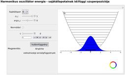
This animation shows the time evolution of the simple harmonic oscillator if it is initially in the superposition of the ground state \((n=0)\) and the \(n=1\) state.
\(\Psi(x, 0)=\frac{1}{\sqrt{2}}\left(\varphi_{0}(x)+\varphi_{1}(x)\right)\)
http://titan.physx.u-szeged.hu/~mmquantum/videok/Harmonikus_oszcillator_szuperpozicio_0_1.flv
This interactive animation gives us a tool to play with the eigenfunctions of the linear harmonic oscillator. We can construct different linear combinations of the energy eigenfunctions and study their evolution in time.
Expectation values and operators
The wave function gives the probability distribution of the position of a particle with the property (2.5). According to probability theory the expectation value or mean value of the position of the particle moving in one dimension is given by
\(\langle\hat{X}\rangle_{\psi}=\int_{-\infty}^{\infty} x|\psi(x)|^{2} d x=\int \psi^{*}(x) x \psi(x) d x\) (2.29)
the reason of writing capital \(\hat{X}\) will be seen below. We did not put the limits deliberately in the second definite integral. In what follows, if the limits are not shown explicitly, then the integration always goes from \(−∞\) to \(+∞\), in one dimension, and over the whole three dimensional space in three dimensions. Therefore in an analogous way for a three-dimensional motion we can define the expectation value of the radius vector as
\(\langle\hat{\mathbf{R}}\rangle_{\psi}=\int \mathbf{r}|\psi(\mathbf{r})|^{2} d^{3} \mathbf{r}=\int \psi^{*}(\mathbf{r}) \mathbf{r} \psi(\mathbf{r}) d^{3} \mathbf{r}\) (2.30)
which actually means three different integrals for each component of \(\mathbf{r}\). Now assume that the particle moves in an external force field given by the potential energy \(V(\mathbf{r})\). If we know only the probability distribution and not the exact value of the particles position we cannot speak either about the value of the potential energy but only about its probability distribution. The expectation value of the potential energy is
\(\langle V(\hat{\mathbf{R}})\rangle_{\psi}=\int \psi^{*}(\mathbf{r}) V(\mathbf{r}) \psi(\mathbf{r}) d^{3} \mathbf{r}\) (2.31)
Note that the expectation value depends on the wave function, i. e on the physical state of the system, in which the quantities are measured. The general expectation value of a measurable quantity, \(\hat{A}\) (which is called sometimes as an observable), is defined as,
\(\langle\hat{A}\rangle_{\psi}=\int \psi^{*}(\mathbf{r}) \hat{A} \psi(\mathbf{r}) d^{3} \mathbf{r}\) (2.32)
where (\hat{A}\) is the operator corresponding to the physical quantity. An operator in the present context is an operation that transforms a square integrable function to another function. According to (2.29) the \(\hat{X}\) operator corresponding to the coordinate multiplies the the wave function with the coordinate x.
\(\hat{X} \Psi(x, t)=x \Psi(x, t)\) (2.33)
Or more generally in three dimensions:
\(\hat{\mathbf{R}} \Psi(\mathbf{r}, t)=\mathbf{r} \Psi(\mathbf{r}, t)\) (2.34)
We may raise the question, what is the operator of the other fundamental quantity, momentum \(\mathbf{p}\). It turns out that the corresponding operator is the derivative of \(ψ\) multiplied by the factor \(\frac{\hbar}{i}\), or equivalently by \(−iℏ\) :
\(\hat{P}_{x} \Psi(x, t)=-i \hbar \frac{\partial}{\partial x} \Psi(x, t)\) (2.35)
\(\hat{\mathbf{P}} \Psi(\mathbf{r}, t)=-i \hbar \nabla \Psi(\mathbf{r}, t)\) (2.36)
Then according to the general rule 2.32 we have in one dimension
\(\left\langle\hat{P}_{x}\right\rangle_{\psi}=-i \hbar \int \psi^{*}(x) \frac{\partial}{\partial x} \psi(x) d x\) (2.37)
A justification of this statement is left to the next series of problems
Using the Schrödinger equation 2.2 prove that with the definitions above one has (in one dimension)
\(\left\langle\hat{P}_{x}\right\rangle_{\psi}=m \frac{d}{d t}\langle\hat{X}\rangle_{\psi}\) (2.38)
Hints:
- Show that the time derivative of the expectation value of the coordinate can be calculated as
\(\frac{d}{d t}\langle\hat{X}\rangle=\frac{\hbar}{2 i m} \int\left(\frac{\partial^{2} \Psi^{*}(x, t)}{\partial x^{2}} x \Psi(x, t)-\Psi^{*}(x, t) x \frac{\partial^{2} \Psi(x, t)}{\partial x^{2}}\right) d x\) (2.39)
- Rewrite the integrand as \(\frac{\partial}{\partial x}\left(\frac{\partial \Psi}{\partial x}^{*} x \Psi-\Psi^{*} x \frac{\partial \Psi}{\partial x}-|\Psi|^{2}\right)+2 \Psi^{*} \frac{\partial \Psi}{\partial x}\), and assuming that \(Ψ(x,t)\) goes to zero at \(±∞\) argue that only the last term contributes to the result.
Show that the expectation value of \(\langle\hat{P}\rangle\) is real.
An operator \(\hat{A}\) is called a self-adjoint or (Hermitian) if the following property holds for square integrable functions \(φ(\mathbf{r})\) and \(ψ(\mathbf{r})\)
\(\int \varphi^{*}(\mathbf{r})[\hat{A} \psi(\mathbf{r})] d^{3} \mathbf{r}=\int[\hat{A} \varphi(\mathbf{r})]^{*} \psi(\mathbf{r}) d^{3} \mathbf{r}\) (2.40)
Show that the components of \(\hat{\mathbf{R}}\) and \(\hat{\mathbf{P}}\) are selfadjoint.
Show that the expectation value of a selfadjoint operator is real.
Noncommutativity of \(\hat{X}\) and \(\hat{P}\) operators
The fact that in quantum mechanics the coordinate and momentum are represented by operators – and they have the form we have given above – implies that their action on a wave function \(Ψ(\mathbf{r},t)\) will give different result if they act on it in a different order:
\(\hat{X} \hat{P}_{x} \Psi(\mathbf{r}, t)-\hat{P}_{x} \hat{X} \Psi(\mathbf{r}, t)=-i \hbar x \frac{\partial}{\partial x} \Psi(\mathbf{r}, t)+i \hbar \frac{\partial}{\partial x}[x \Psi(\mathbf{r}, t)]=i \hbar \Psi(\mathbf{r}, t)\) (2.41)
or written in another way:
\((\hat{X} \hat{P}-\hat{P} \hat{X}) \Psi(\mathbf{r}, t)=i \hbar \Psi(\mathbf{r}, t)\) (2.42)
for any function. This means that the action of the two operators are different, if they are taken in the reverse order, so this pair of operators is noncommutative. It is easily seen, that the same is true for Y and \(\hat{P}_{y}\) and for \(\hat{Z}\) and \(\hat{P}_{z}\), while say \(\hat{X}\) and \(\hat{P}_{y}\) do commute, because the partial derivation by y gives zero for x. Similarly the components of \(\hat{\mathbf{R}}\) among themselves as well as the components of \(\hat{\mathbf{P}}\) among themselves commute with each other. Introducing the notation
\(\hat{X} \hat{P}_{x}-\hat{P}_{x} \hat{X}=:\left[\hat{X}, \hat{P}_{x}\right]\) (2.43)
which is called the commutator of the operators \(\hat{X}\) and \(\hat{P}_{x}\), we see that the commutator vanishes if the operators commute, and it is nonzero if this is not the case. To summarize we write down here the following canonical commutation relations:
\(\left[\hat{X}_{i}, \hat{X}_{j}\right]=0, \quad\left[\hat{P}_{i}, \hat{P}_{j}\right]=0, \quad\left[\hat{X}_{i}, \hat{P}_{j}\right]=i \hbar \delta_{i j}\) (2.44)
From the operators of the coordinate and the momentum we can build up other operators depending on these quantities. The rule is that in the classical expression of a function of \(\mathbf{r}\) and \(\mathbf{p}\) we replace them by the corresponding operators. We will see for instance that the operator of orbital angular momentum \(\hat{\mathbf{L}}=\hat{\mathbf{R}} \times \hat{\mathbf{P}}=-i \hbar \mathbf{r} \times \nabla\), and the operator of energy in a conservative system is \(\hat{H}=\frac{\hat{\mathbf{p}}^{2}}{2 m}+V(\hat{\mathbf{R}})=-\frac{\hbar^{2}}{2 m} \Delta+V(r)\) in agreement with the definition given in (2.4)
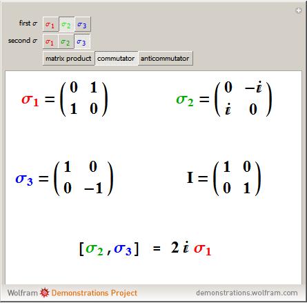
Non commutativity arise also in case of matrix multiplication. This demonstration shows non commutativity in case of special 2×22×2 complex matrices, the so called Pauli matrices.
Variance of an operator
There is an important number characterising a probability distribution, which is the property showing how sharp the distribution is. A measure of this property can be obtained, if we take the measured values of the random variable in question, and consider a mean value of certain differences between the measured values and the expectation value. As an example we consider again the one dimensional coordinate x. Taking the expectation value of the simple differences between the measured values and the expectation yields no information, as this gives zero in cases of all possible distributions due to the identity: \(\int_{-\infty}^{\infty}\left[x^{\prime}-\int_{-\infty}^{\infty} x|\psi(x)|^{2} d x\right]\left|\psi\left(x^{\prime}\right)\right|^{2} d x^{\prime}=0\). A good measure is therefore to take the expectation value of the square of the differences from the expectation value, i.e. the quantity:
\((\Delta \hat{X})_{\psi}^{2}:=\int_{-\infty}^{\infty}\left[x^{\prime}-\int_{-\infty}^{\infty} x|\psi(x)|^{2} d x\right]^{2}\left|\psi\left(x^{\prime}\right)\right|^{2} d x^{\prime}\) (2.45)
which is called the variance of x, and which is the usual definition in probability theory, with a probability density \(|\psi(x)|^{2}=\rho(x)\). We shall also call this the variance of the operator \(\hat{X}\) in the state \(ψ\). The latter terminology is due to the reformulation of the above definition as:
\((\Delta \hat{X})_{\psi}^{2}=\left\langle\left(\hat{X}-\langle\hat{X}\rangle_{\psi}\right)^{2}\right\rangle_{\psi}\) (2.46)
or in general for any linear and selfadjoint operator (2.32).
\((\Delta \hat{A})_{\psi}^{2}=\left\langle\left(\hat{A}-\langle\hat{A}\rangle_{\psi}\right)^{2}\right\rangle_{\psi}\) (2.47)
The variance is also called the second central moment of the probability distribution. The square root \(\sqrt{(\Delta \hat{A})_{\psi}^{2}}=:(\Delta \hat{A})_{\psi}\) is called the root mean square deviation of the physical quantity \(\hat{A}\) in the state given by \(ψ\). We can rewrite this formula in two different ways. First it is simply seen that
\((\Delta \hat{A})_{\psi}^{2}=\left\langle\hat{A}^{2}-2 \hat{A}\langle\hat{A}\rangle_{\psi}+\langle\hat{A}\rangle_{\psi}^{2}\right\rangle_{\psi}=\left\langle\hat{A}^{2}\right\rangle_{\psi}-\langle\hat{A}\rangle_{\psi}^{2}\) (2.48)
because \(\langle\hat{A}\rangle_{\psi}/) is already a number. An important statement follows if we write
\(\begin{aligned}
(\Delta \hat{A})_{\psi}^{2} &=\left\langle\left(\hat{A}-\langle\hat{A}\rangle_{\psi}\right)^{2}\right\rangle_{\psi}=\int \psi^{*}(\mathbf{r})\left(\hat{A}-\langle\hat{A}\rangle_{\psi}\right)^{2} \psi(\mathbf{r}) d^{3} \mathbf{r}=\\
&\left.=\int\left[\left(\hat{A}-\langle\hat{A}\rangle_{\psi}\right) \psi(\mathbf{r})\right]^{*}\left[\left(\hat{A}-\langle\hat{A}\rangle_{\psi}\right) \psi(\mathbf{r})\right] d^{3} \mathbf{r}=\int \mid \hat{A}-\langle\hat{A}\rangle_{\psi} \psi(\mathbf{r})\right)\left.\right|^{2} d^{3} \mathbf{r}
\end{aligned}\) (2.49)
Based on this formula, we can simply answer the question: what kind of wave functions are those, where we can measure the quantity corresponding to \(\hat{A}\) with zero variance, i.e. with a value which is always the same? In order to have \((\Delta \hat{A})_{\psi}^{2}=0\) the integral in the last expression must be zero. But as it is an integral of a squared absolute value being nonnegative everywhere, it can be zero if and only if \(\left(\hat{A}-\langle\hat{A}\rangle_{\psi}\right) \psi(\mathbf{r})=0\), or stated otherwise, if and only if
\(\hat{A} \psi(\mathbf{r})=\langle\hat{A}\rangle_{\psi} \psi(\mathbf{r})\) (2.50)
Any function obeying this equation is called the eigenfunction of the operator \(\hat{A}\). In the form above this equation has only a principal significance and in most cases knowing the operator, the eigenfunctions are not known a priori. Therefore the problem is usually to determine the eigenvalues and the eigenfunctions of \(\hat{A}\) from the equation:
\(\hat{A} \varphi(\mathbf{r})=\alpha \varphi(\mathbf{r})\) (2.51)
This was the case above, in particular, for the Hamilton operator in (2.12).
Show that the expectation value of \(\hat{A}\) in the state given by the normalized \(φ(r)\), is just α.
An important theorem shows that the product of variances of two noncommuting operators has a lower bound, which is generally positive. In the case of the coordinate and momentum operators it takes the form
\((\Delta \hat{X})_{\psi} \cdot\left(\Delta \hat{P}_{x}\right)_{\psi} \geq \frac{\hbar}{2}\) (2.52)
for any wave function \(ψ\), and a similar inequality holds for the other two \((y,z)\) components. The mathematical proof of the inequality, which is called customarily as Heisenberg’s uncertainty relation, will not be given here


