
3: Angular momentum in quantum mechanics


- Last updated
- Oct 30, 2021
- Save as PDF

( \newcommand{\kernel}{\mathrm{null}\,}\)
In this chapter we discuss the angular momentum operator – one of several related operators – analogous to classical angular momentum. The angular momentum operator plays a central role in the theory of atomic physics and other quantum problems involving rotational symmetry. In both classical and quantum mechanical systems, angular momentum (together with linear momentum and energy) is one of the three fundamental properties of motion.
Chapters 1 and 2. Angular momentum and its conservation in classical mechanics. Spherical coordinates, elements of vector analysis. Laplace equation.
Eigenvalue equation in polar coordinates
The classical definition of the angular momentum vector is
L=r×p (3.1)
which depends on the choice of the point of origin where |r|=r=0|r|=r=0. With the definition of the position and the momentum operators we obtain the angular momentum operator as
ˆL=−iℏ(r×∇) (3.2)
The Cartesian components of ˆL are then
ˆLx=−iℏ(y∂z−z∂y),ˆLy=−iℏ(z∂x−x∂z),ˆLz=−iℏ(x∂y−y∂x) (3.3)
One frequently needs the components of ˆL in spherical coordinates. In order to obtain them we have to make use of the expression of the position vector by spherical coordinates, which are connected to the Cartesian components by
r=xˆex+yˆey+zˆez=rsinθcosϕˆex+rsinθsinϕˆey+rcosθˆez (3.4)
Going over to the spherical components in (3.3), and using the chain rule:
∂x=(∂xr)∂r+(∂xθ)∂θ+(∂xϕ)∂ϕ (3.5)
and similarly for ∂y and ∂z gives the following components
ˆLx=iℏ(sinϕ∂θ+cotθcosϕ∂ϕ)ˆLy=iℏ(−cosϕ∂θ+cotθsinϕ∂ϕ)ˆLz=−iℏ∂ϕ (3.6)
One sees at once the reason and the advantage of using spherical coordinates: the operators in question do not depend on the radial variable r. This is of course also true for ˆL2=ˆL2x+ˆL2y+ˆL2z which turns out to be −ℏ^{2} times the angular part of the Laplace operator Δ_{θϕ}.
\hat{L}^{2}=-\hbar^{2}\left(\partial_{\theta \theta}^{2}+\cot \theta \partial_{\theta}+\frac{1}{\sin ^{2} \theta} \partial_{\phi \phi}^{2}\right)=-\hbar^{2} \Delta_{\theta \phi} (3.7)
We shall now find the eigenfunctions of Δ_{θϕ}, that play a very important role in quantum mechanics, and actually in several branches of theoretical physics. They will be functions of 0 \leq \theta \leq \pi and 0 \leq \phi<2 \pi, i.e. they can be considered as complex valued functions whose domain is the unit sphere. The eigenfunctions of \hat{L}^{2} will be denoted by Y(θ,ϕ), and the angular eigenvalue equation is:
\begin{aligned} -\Delta_{\theta \phi} Y(\theta, \phi) &=\ell(\ell+1) Y(\theta, \phi) \quad \text { or } \\ \left(\partial_{\theta \theta}^{2}+\cot \theta \partial_{\theta}+\frac{1}{\sin ^{2} \theta} \partial_{\phi \phi}^{2}\right) Y(\theta, \phi) &=-\ell(\ell+1) Y(\theta, \phi) \end{aligned} (3.8)
One might wonder what is the reason for writing the eigenvalue in the form ℓ(ℓ+1), but as it will turn out soon, there is no loss of generality in this notation.
Separation of the eigenvalue equation
We try the separation of the variables:
Y(\theta, \phi)=\Theta(\theta) \Phi(\phi) (3.9)
Plugging this into (3.8) and dividing by ΘΦ, we find
\left\{\frac{1}{\Theta}\left[\sin \theta \frac{d}{d \theta}\left(\sin \theta \frac{d \Theta}{d \theta}\right)\right]+\ell(\ell+1) \sin ^{2} \theta\right\}+\frac{1}{\Phi} \frac{d^{2} \Phi}{d \phi^{2}}=0 (3.10)
The first term depends only on θ while the last one is a function of only ϕ. In order to satisfy this equation for all values of θ and ϕ these terms must be separately equal to a constant with opposite signs. This constant is traditionally denoted by m^{2} and −m^{2} (note that this is not the mass) and we have two equations: one for Θ, and another for Φ. We consider the second one, and have:
\frac{1}{\Phi} \frac{d^{2} \Phi}{d \phi^{2}}=-m^{2} (3.11)
Two linearly independent solutions are
\Phi(\phi)=\left\{\begin{array}{l} e^{i m \phi} \\ e^{-i m \phi} \end{array}\right. (3.12)
and any linear combinations of them. One can choose e^{imϕ}, and include the other one by allowing mm to be negative. As these are functions of points in real three dimensional space, the values of Φ(ϕ) and Φ(ϕ+2π) must be the same, as these values of the argument correspond to identical points in space. Then e^{im(ϕ+2π)}=e^{imϕ}, and e^{im2π}=1 must hold. From this it follows that mm must be an integer
\Phi(\phi)=\frac{1}{\sqrt{2 \pi}} e^{i m \phi} \quad m=0, \pm 1, \pm 2 \ldots (3.15)
The integration constant \frac{1}{\sqrt{2 \pi}} has been chosen here so that already Φ(ϕ) is normalized to unity when integrating with respect to ϕ from 0 to 2π.
The equation for Θ
\sin \theta \frac{d}{d \theta}\left(\sin \theta \frac{d \Theta}{d \theta}\right)+\left[\ell(\ell+1) \sin ^{2} \theta-m^{2}\right] \Theta=0 (3.16)
is more complicated. With \cos \theta=z the solution is
P_{\ell}^{m}(z):=\left(1-z^{2}\right)^{|m| 2}\left(\frac{d}{d z}\right)^{|m|} P_{\ell}(z) (3.17)
where P_{ℓ}(z) is the ℓ-th Legendre polynomial, defined by the following formula, (called the Rodrigues formula):
P_{\ell}(z):=\frac{1}{2^{\ell} \ell !}\left(\frac{d}{d z}\right)^{\ell}\left(z^{2}-1\right)^{\ell} (3.18)
The functions P_{\ell}^{m}(z) are called associated Legendre functions.
Find the first three Legendre polynomials P_{0}(z), P_{1}(z) and P_{2}(z).
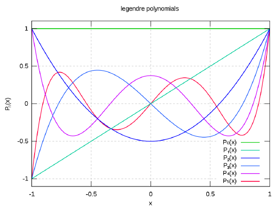
Figure 3.1: Plot of the first six Legendre polynomials.
http://en.Wikipedia.org/wiki/File:Legendrepolynomials6.svg
The function P_{\ell}^{m}(z) is a polynomial in z only if |m| is even, otherwise it contains a term \left(1-z^{2}\right)^{|m| / 2} which is a square root. But when turning back to cosθ=z this factor reduces to (\sin \theta)^{|m|}.
Find P_{2}^{0}(\theta), P_{2}^{1}(\theta), P_{2}^{2}(\theta).
Prove that P_{ℓ}(z) are solutions of (3.16) for m=0.
Prove that P_{\ell}^{m}(z) are solutions of (3.16) for all ℓ and |m|, if |m|≤ℓ.
Show that P_{ℓ}(z) are either even, or odd depending on the parity of ℓ.
Notice that ℓ must be a nonnegative integer otherwise the definition (3.18) makes no sense, and in addition if |(|m|>ℓ\), then (3.17) yields zero. Thus for any given ℓ, there are 2ℓ+1 allowed values of m:
m=-\ell,-\ell+1, \ldots-1,0,1, \ldots \ell-1, \ell, \quad \text { for } \quad \ell=0,1,2, \ldots (3.19)
Note that equation (3.16) – as all second order differential equations – must have other linearly independent solutions different from P_{\ell}^{m}(z) for a given value of ℓ and m. One can show however, that these latter solutions are divergent for θ=0 and θ=π, and therefore they are not describing physical states. The solutions
Y_{\ell}^{m}(\theta, \phi)=\mathcal{N}_{l m} P_{\ell}^{m}(\theta) e^{i m \phi} (3.20)
where the absolute values of the constants \mathcal{N}_{l m} ensure the normalization over the unit sphere, are called spherical harmonics. There are several different conventions for the phases of \mathcal{N}_{l m}, so one has to be careful with them.
The Y_{\ell}^{m}(\theta) functions are thus the eigenfunctions of \hat{L} corresponding to the eigenvalue \hbar^{2} \ell(\ell+1), and they are also eigenfunctions of \hat{L}_{z}=-i \hbar \partial_{\phi}, because
\hat{L}_{z} Y_{\ell}^{m}(\theta, \phi)=-i \hbar \partial_{\phi} Y_{\ell}^{m}(\theta, \phi)=\hbar m Y_{\ell}^{m}(\theta, \phi) (3.21)
The quantum number ℓ is called angular momentum quantum number, or sometimes for a historical reason as azimuthal quantum number, while m is the magnetic quantum number.
Concluding the subsection let us note the following important fact. As none of the components of \mathbf{\hat{L}}, and thus nor \hat{L}^{2} depends on the radial distance rr from the origin, then any function of the form \mathcal{R}(r) Y_{\ell}^{m}(\theta, \phi) will be the solution of the eigenvalue equation above, because from the point of view of the \mathbf{\hat{L}} the \mathcal{R}(r) function is a constant, and we can freely multiply both sides of (3.8). by \mathcal{R}(r).
Orthonormality and completeness
The spherical harmonics form an infinite system of orthonormal functions in the sense:
\int_{0}^{2 \pi} \int_{0}^{\pi}\left(Y_{\ell^{\prime}}^{m^{\prime}}(\theta, \phi)\right)^{*} Y_{\ell}^{m}(\theta, \phi) \sin \theta d \theta d \phi=\delta_{\ell \ell^{\prime}} \delta_{m m^{\prime}} (3.22)
This system is also a complete one, which means that any complex valued function g(θ,ϕ) that is square integrable on the unit sphere, i.e. \int|g(\theta, \phi)|^{2} \sin \theta d \theta d \phi<\infty can be expanded in terms of the Y_{\ell}^{m}(\theta, \phi)):
g(\theta, \phi)=\sum_{\ell=0}^{\infty} \sum_{m=-\ell}^{\ell} c_{\ell m} Y_{\ell}^{m}(\theta, \phi) (3.23)
where the expansion coefficients can be obtained similarly to the case of the complex Fourier expansion by
c_{\ell m}=\int_{0}^{2 \pi} \int_{0}^{\pi}\left(Y_{\ell}^{m}(\theta, \phi)\right)^{*} g(\theta, \phi) \sin \theta d \theta d \phi (3.24)
If you are interested in the topic Spherical harmonics in more details check out the Wikipedia link below:
http://en.Wikipedia.org/wiki/Spherical_harmonics
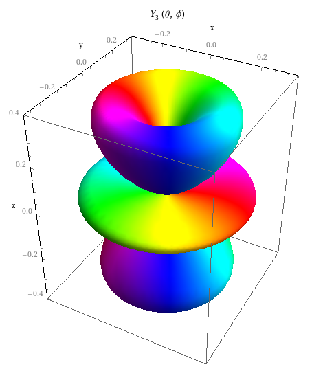
The animation shows the time dependence of the stationary state – i.e. the one containing the time dependent factor e_{−iϵt/ℏ} as well – given by the function Y_{1}^{3}(θ,ϕ). The absolute value of the function in the direction given by θ and ϕ is equal to the distance of the point from the origin, and the argument of the complex number is obtained by the colours of the surface according to the phase code of the complex number in the chosen direction.
http://titan.physx.u-szeged.hu/~mmquantum/videok/Gombfuggveny_fazis_idofejlodes.flv
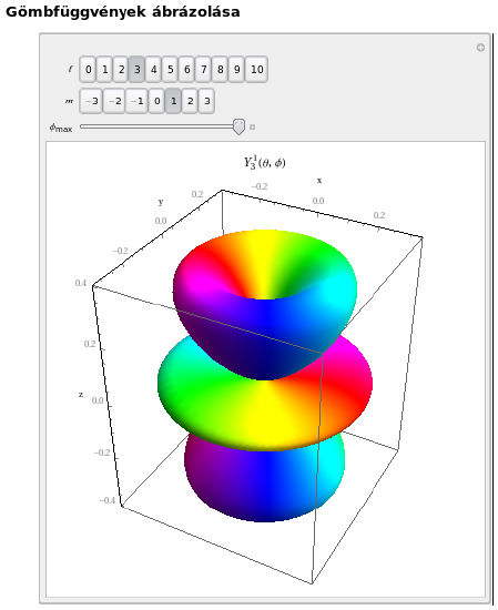
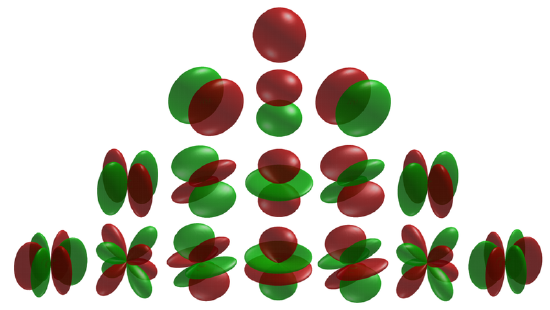
The figures show the three-dimensional polar diagrams of the spherical harmonics. The state to be shown, can be chosen by setting the quantum numbers ℓ and m.
http://titan.physx.u-szeged.hu/~mmquantum/interactive/Gombfuggvenyek.nbp
Specific examples
The first few functions are the following, with one of the usual phase (sign) conventions:
Y_{0}^{0}(\theta, \phi)=\frac{1}{\sqrt{4} \pi} (3.25)
Y_{1}^{0}(\theta, \phi)=\sqrt{\frac{3}{4 \pi}} \cos \theta, \quad Y_{1}^{1}(\theta, \phi)=-\sqrt{\frac{3}{8 \pi}} \sin \theta e^{i \phi}, \quad Y_{1}^{-1}(\theta, \phi)=\sqrt{\frac{3}{8 \pi}} \sin \theta e^{-i \phi} (3.26)
Historically the spherical harmonics with the labels ℓ=0,1,2,3,4 are called s, p, d, f, g \ldots functions respectively, the terminology is coming from spectroscopy.
If an external magnetic field \mathbf{B}=\{0,0, B\} is applied, the projection of the angular momentum onto the field direction is ℏm. Since mm can take only the integer values between −ℓ and +ℓ, there are 2ℓ+1 different possible projections, corresponding to the 2ℓ+1 different functions Y_{m}^{ℓ}(θ,ϕ) with a given ℓ.
Very often the spherical harmonics are given by Cartesian coordinates by exploiting \sin \theta e^{\pm i \phi}=(x \pm i y) / r and \cos \theta=z / r. Another way of using these functions is to create linear combinations of functions with opposite m-s. This is useful for instance when we illustrate the orientation of chemical bonds in molecules. We demonstrate this with the example of the p functions.
\begin{aligned} &p_{x}=\frac{x}{r}=\frac{\left(Y_{1}^{-1}-Y_{1}^{1}\right)}{\sqrt{2}}=\sqrt{\frac{3}{4 \pi}} \sin \theta \cos \phi \\ &p_{x}=\frac{y}{r}=-\frac{\left(Y_{1}^{-1}+Y_{1}^{1}\right)}{\sqrt{2}}=\sqrt{\frac{3}{4 \pi}} \sin \theta \sin \phi \\ &p_{z}=\frac{z}{r}=Y_{1}^{0}=\sqrt{\frac{3}{4 \pi}} \cos \theta \end{aligned} (3.27)
Let us also note that the m=0 functions do not depend on ϕ, and they are proportional to the Legendre polynomials in cosθ.
Y_{\ell}^{0}(\theta)=\sqrt{\frac{2 \ell+1}{4 \pi}} P_{\ell}(\cos \theta) (3.28)
Parity and angular momentum
The operator of parity Π is defined in the following way:
\Pi \psi(\mathbf{r})=\psi(-\mathbf{r}) (3.29)
The result of acting by the parity on a function is the mirror image of the original function with respect to the origin. Looking for the eigenvalues and eigenfunctions of Π, we note first that Π^{2}=1. Therefore the single eigenvalue of Π^{2} is 1, and any function is its eigenfunction. The eigenvalues of Π itself are then ±1, and we have the following two possibilities:
\begin{aligned} &\Pi_{\psi_{+}}(\mathbf{r})=\quad \psi_{+}(-\mathbf{r})=\psi_{+}(\mathbf{r}) \\ &\Pi_{\psi_{-}}(\mathbf{r})=\quad \psi_{-}(-\mathbf{r})=-\psi_{-}(\mathbf{r}) \end{aligned} (3.30)
In the first case the eigenfunctions \psi_{+}(\mathbf{r}) belonging to eigenvalue +1 are the even functions, while in the second we see that \psi_{-}(\mathbf{r}) are the odd functions belonging to the eigenvalue −1. There are of course functions which are neither even nor odd, they do not belong to the set of eigenfunctions of Π.
The reason why we consider parity in connection with the angular momentum is that the simultaneous eigenfunctions of \hat{L}^{2} and \hat{L}_{z} the spherical harmonics times any function of the radial variable r are eigenfunctions of Π as well, and the corresponding eigenvalues are (−1)^{ℓ}. This can be formulated as:
\Pi \mathcal{R}(r) Y_{\ell}^{m}(\theta, \phi)=\mathcal{R}(r) \Pi Y_{\ell}^{m}(\theta, \phi)=(-1)^{\ell} \mathcal{R}(r) Y(\theta, \phi) (3.31)
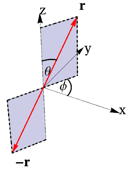
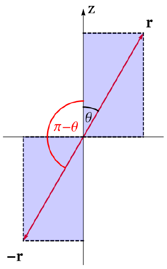
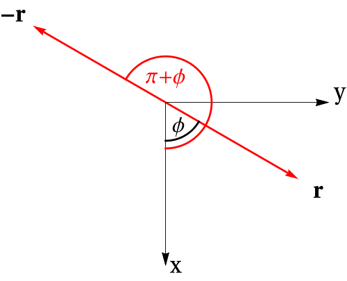
Show that the transformation \{x, y, z\} \longrightarrow\{-x,-y,-z\} is equivalent to \theta \longrightarrow \pi-\theta, \quad \phi \longrightarrow \phi+\pi.
By using the results of the previous subsections prove the validity of Eq. (3.31).