2.3: Representation of Waves via Complex Functions

In mathematics, the symbol \({\rm i}\) is conventionally used to represent the square-root of minus one: in other words, one of the solutions of \({\rm i}^2 = -1\). Now, a real number, \(x\) (say), can take any value in a continuum of different values lying between \(-\infty\) and \(+\infty\). On the other hand, an imaginary number takes the general form \({\rm i}\,y\), where \(y\) is a real number. It follows that the square of a real number is a positive real number, whereas the square of an imaginary number is a negative real number. In addition, a general complex number is written

\[z = x + {\rm i}\,y, \nonumber \]

where \(x\) and \(y\) are real numbers. In fact, \(x\) is termed the real part of \(z\), and \(y\) the imaginary part of \(z\). This is written mathematically as \(x={\rm Re}(z)\) and \(y={\rm Im}(z)\). Finally, the complex conjugate of \(z\) is defined \(z^\ast = x-{\rm i}\,y\).

Just as we can visualize a real number as a point lying on an infinite straight-line, we can visualize a complex number as a point lying in an infinite plane. The coordinates of the point in question are the real and imaginary parts of the number: that is, \(z\equiv (x,\,y)\). This idea is illustrated in Figure [f13.2]. The distance, \(r=(x^2+y^2)^{1/2}\), of the representative point from the origin is termed the modulus of the corresponding complex number, \(z\). This is written mathematically as \(|z|=(x^2+y^2)^{1/2}\). Incidentally, it follows that \(z\,z^\ast = x^2 + y^2=|z|^2\). The angle, \(\theta=\tan^{-1}(y/x)\), that the straight-line joining the representative point to the origin subtends with the real axis is termed the argument of the corresponding complex number, \(z\). This is written mathematically as \({\rm arg}(z)=\tan^{-1}(y/x)\). It follows from standard trigonometry that \(x=r\,\cos\theta\), and \(y=r\,\sin\theta\). Hence, \(z= r\,\cos\theta+ {\rm i}\,r\sin\theta\).

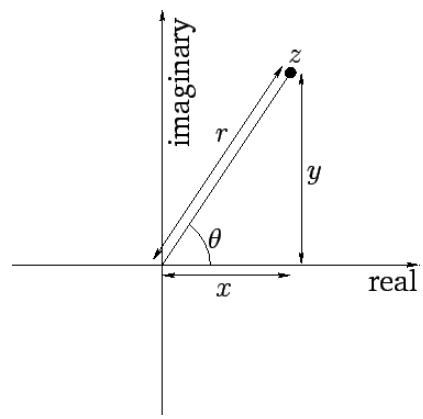
Figure 3: Representation of a complex number as a point in a plane.

Complex numbers are often used to represent wavefunctions. All such representations depend ultimately on a fundamental mathematical identity, known as Euler’s theorem , that takes the form

\[\rm e^{\,{\rm i}\,\phi} \equiv \cos\phi + {\rm i}\,\sin\phi, \nonumber \]

where \(\phi\) is a real number. Incidentally, given that \(z=r\,\cos\theta + {\rm i}\,r\,\sin\theta= r\,(\cos\theta+{\rm i}\,\sin\theta)\), where \(z\) is a general complex number, \(r=|z|\) its modulus, and \(\theta={\rm arg}(z)\) its argument, it follows from Euler’s theorem that any complex number, \(z\), can be written

\[z = r\,\rm e^{\,{\rm i}\,\theta}, \nonumber \]

where \(r=|z|\) and \(\theta={\rm arg}(z)\) are real numbers.

A one-dimensional wavefunction takes the general form

\[ \psi(x,t) = A\,\cos(k\,x-\omega\,t+\varphi), \label{e12.8} \]

where \(A\) is the wave amplitude, \(k\) the wavenumber, \(\omega\) the angular frequency, and \(\varphi\) the phase angle. Consider the complex wavefunction

\[ \psi(x,t) = \psi_0\,\rm e^{\,{\rm i}\,(k\,x-\omega\,t)}, \label{e12.10} \]

where \(\psi_0\) is a complex constant. We can write

\[\psi_0 = A\,\rm e^{\,{\rm i}\,\varphi}, \nonumber \]

where \(A\) is the modulus, and \(\varphi\) the argument, of \(\psi_0\). Hence, we deduce that

\[\begin{align} {\rm Re}\left[\psi_0\,\rm e^{\,{\rm i}\,(k\,x-\omega\,t)}\right] &= {\rm Re}\left[A\,\rm e^{\,{\rm i}\,\varphi}\,\rm e^{\,{\rm i}\,(k\,x-\omega\,t)}\right]={\rm Re}\left[A\,\rm e^{\,{\rm i}\,(k\,x-\omega\,t+\varphi)}\right]=A\,{\rm Re}\left[\rm e^{\,{\rm i}\,(k\,x-\omega\,t+\varphi)}\right].\end{align} \nonumber \]

Thus, it follows from Euler’s theorem, and Equation \ref{e12.8}, that

\[{\rm Re}\left[\psi_0\,\rm e^{\,{\rm i}\,(k\,x-\omega\,t)}\right] =A\,\cos(k\,x-\omega\,t+\varphi)=\psi(x,t). \nonumber \]

In other words, a general one-dimensional real wavefunction, \ref{e12.8}, can be represented as the real part of a complex wavefunction of the form \ref{e12.10}. For ease of notation, the “take the real part” aspect of the previous expression is usually omitted, and our general one-dimension wavefunction is simply written

\[ \psi(x,t) = \psi_0\,\rm e^{\,{\rm i}\,(k\,x-\omega\,t)}. \label{e12.13} \]

The main advantage of the complex representation, \ref{e12.13}, over the more straightforward real representation, \ref{e12.8}, is that the former enables us to combine the amplitude, \(A\), and the phase angle, \(\varphi\), of the wavefunction into a single complex amplitude, \(\psi_0\). Finally, the three-dimensional generalization of the previous expression is

\[\psi({\bf r},t) = \psi_0\,\rm e^{\,{\rm i}\,({\bf k}\cdot{\bf r}-\omega\,t)}, \nonumber \]

where \({\bf k}\) is the wavevector.