2.12: Schrodinger's Equation and Wavefunction Collapse
- Page ID
- 16027
\( \newcommand{\vecs}[1]{\overset { \scriptstyle \rightharpoonup} {\mathbf{#1}} } \)
\( \newcommand{\vecd}[1]{\overset{-\!-\!\rightharpoonup}{\vphantom{a}\smash {#1}}} \)
\( \newcommand{\dsum}{\displaystyle\sum\limits} \)
\( \newcommand{\dint}{\displaystyle\int\limits} \)
\( \newcommand{\dlim}{\displaystyle\lim\limits} \)
\( \newcommand{\id}{\mathrm{id}}\) \( \newcommand{\Span}{\mathrm{span}}\)
( \newcommand{\kernel}{\mathrm{null}\,}\) \( \newcommand{\range}{\mathrm{range}\,}\)
\( \newcommand{\RealPart}{\mathrm{Re}}\) \( \newcommand{\ImaginaryPart}{\mathrm{Im}}\)
\( \newcommand{\Argument}{\mathrm{Arg}}\) \( \newcommand{\norm}[1]{\| #1 \|}\)
\( \newcommand{\inner}[2]{\langle #1, #2 \rangle}\)
\( \newcommand{\Span}{\mathrm{span}}\)
\( \newcommand{\id}{\mathrm{id}}\)
\( \newcommand{\Span}{\mathrm{span}}\)
\( \newcommand{\kernel}{\mathrm{null}\,}\)
\( \newcommand{\range}{\mathrm{range}\,}\)
\( \newcommand{\RealPart}{\mathrm{Re}}\)
\( \newcommand{\ImaginaryPart}{\mathrm{Im}}\)
\( \newcommand{\Argument}{\mathrm{Arg}}\)
\( \newcommand{\norm}[1]{\| #1 \|}\)
\( \newcommand{\inner}[2]{\langle #1, #2 \rangle}\)
\( \newcommand{\Span}{\mathrm{span}}\) \( \newcommand{\AA}{\unicode[.8,0]{x212B}}\)
\( \newcommand{\vectorA}[1]{\vec{#1}} % arrow\)
\( \newcommand{\vectorAt}[1]{\vec{\text{#1}}} % arrow\)
\( \newcommand{\vectorB}[1]{\overset { \scriptstyle \rightharpoonup} {\mathbf{#1}} } \)
\( \newcommand{\vectorC}[1]{\textbf{#1}} \)
\( \newcommand{\vectorD}[1]{\overrightarrow{#1}} \)
\( \newcommand{\vectorDt}[1]{\overrightarrow{\text{#1}}} \)
\( \newcommand{\vectE}[1]{\overset{-\!-\!\rightharpoonup}{\vphantom{a}\smash{\mathbf {#1}}}} \)
\( \newcommand{\vecs}[1]{\overset { \scriptstyle \rightharpoonup} {\mathbf{#1}} } \)
\(\newcommand{\longvect}{\overrightarrow}\)
\( \newcommand{\vecd}[1]{\overset{-\!-\!\rightharpoonup}{\vphantom{a}\smash {#1}}} \)
\(\newcommand{\avec}{\mathbf a}\) \(\newcommand{\bvec}{\mathbf b}\) \(\newcommand{\cvec}{\mathbf c}\) \(\newcommand{\dvec}{\mathbf d}\) \(\newcommand{\dtil}{\widetilde{\mathbf d}}\) \(\newcommand{\evec}{\mathbf e}\) \(\newcommand{\fvec}{\mathbf f}\) \(\newcommand{\nvec}{\mathbf n}\) \(\newcommand{\pvec}{\mathbf p}\) \(\newcommand{\qvec}{\mathbf q}\) \(\newcommand{\svec}{\mathbf s}\) \(\newcommand{\tvec}{\mathbf t}\) \(\newcommand{\uvec}{\mathbf u}\) \(\newcommand{\vvec}{\mathbf v}\) \(\newcommand{\wvec}{\mathbf w}\) \(\newcommand{\xvec}{\mathbf x}\) \(\newcommand{\yvec}{\mathbf y}\) \(\newcommand{\zvec}{\mathbf z}\) \(\newcommand{\rvec}{\mathbf r}\) \(\newcommand{\mvec}{\mathbf m}\) \(\newcommand{\zerovec}{\mathbf 0}\) \(\newcommand{\onevec}{\mathbf 1}\) \(\newcommand{\real}{\mathbb R}\) \(\newcommand{\twovec}[2]{\left[\begin{array}{r}#1 \\ #2 \end{array}\right]}\) \(\newcommand{\ctwovec}[2]{\left[\begin{array}{c}#1 \\ #2 \end{array}\right]}\) \(\newcommand{\threevec}[3]{\left[\begin{array}{r}#1 \\ #2 \\ #3 \end{array}\right]}\) \(\newcommand{\cthreevec}[3]{\left[\begin{array}{c}#1 \\ #2 \\ #3 \end{array}\right]}\) \(\newcommand{\fourvec}[4]{\left[\begin{array}{r}#1 \\ #2 \\ #3 \\ #4 \end{array}\right]}\) \(\newcommand{\cfourvec}[4]{\left[\begin{array}{c}#1 \\ #2 \\ #3 \\ #4 \end{array}\right]}\) \(\newcommand{\fivevec}[5]{\left[\begin{array}{r}#1 \\ #2 \\ #3 \\ #4 \\ #5 \\ \end{array}\right]}\) \(\newcommand{\cfivevec}[5]{\left[\begin{array}{c}#1 \\ #2 \\ #3 \\ #4 \\ #5 \\ \end{array}\right]}\) \(\newcommand{\mattwo}[4]{\left[\begin{array}{rr}#1 \amp #2 \\ #3 \amp #4 \\ \end{array}\right]}\) \(\newcommand{\laspan}[1]{\text{Span}\{#1\}}\) \(\newcommand{\bcal}{\cal B}\) \(\newcommand{\ccal}{\cal C}\) \(\newcommand{\scal}{\cal S}\) \(\newcommand{\wcal}{\cal W}\) \(\newcommand{\ecal}{\cal E}\) \(\newcommand{\coords}[2]{\left\{#1\right\}_{#2}}\) \(\newcommand{\gray}[1]{\color{gray}{#1}}\) \(\newcommand{\lgray}[1]{\color{lightgray}{#1}}\) \(\newcommand{\rank}{\operatorname{rank}}\) \(\newcommand{\row}{\text{Row}}\) \(\newcommand{\col}{\text{Col}}\) \(\renewcommand{\row}{\text{Row}}\) \(\newcommand{\nul}{\text{Nul}}\) \(\newcommand{\var}{\text{Var}}\) \(\newcommand{\corr}{\text{corr}}\) \(\newcommand{\len}[1]{\left|#1\right|}\) \(\newcommand{\bbar}{\overline{\bvec}}\) \(\newcommand{\bhat}{\widehat{\bvec}}\) \(\newcommand{\bperp}{\bvec^\perp}\) \(\newcommand{\xhat}{\widehat{\xvec}}\) \(\newcommand{\vhat}{\widehat{\vvec}}\) \(\newcommand{\uhat}{\widehat{\uvec}}\) \(\newcommand{\what}{\widehat{\wvec}}\) \(\newcommand{\Sighat}{\widehat{\Sigma}}\) \(\newcommand{\lt}{<}\) \(\newcommand{\gt}{>}\) \(\newcommand{\amp}{&}\) \(\definecolor{fillinmathshade}{gray}{0.9}\)We have seen that the wavefunction of a free particle of mass \(m\) satisfies \[\label{e2.78} \psi(x,t)=\int_{-\infty}^{\infty}\bar{\psi}(k)\,{\rm e}^{\,{\rm i}\,(k\,x-\omega\,t)}\,dk,\] where \(\bar{\psi}(k)\) is determined by \(\psi(x,0)\), and \[\label{e2.79} \omega(k) = \frac{\hbar\,k^{\,2}}{2\,m}.\] It follows from Equation ([e2.78]) that \[\label{e2.80} \frac{\partial\psi}{\partial x} = \int_{-\infty}^{\infty}({\rm i}\,k)\,\bar{\psi}(k)\,{\rm e}^{\,{\rm i}\,(k\,x-\omega\,t)}\,dk,\] and \[\frac{\partial^{\,2}\psi}{\partial x^{\,2}} = \int_{-\infty}^{\infty}(-k^{\,2})\,\bar{\psi}(k)\,{\rm e}^{\,{\rm i}\,(k\,x-\omega\,t)}\,dk,\] whereas \[\frac{\partial \psi}{\partial t} = \int_{-\infty}^{\infty}(-{\rm i}\,\omega)\,\bar{\psi}(k)\,{\rm e}^{\,{\rm i}\,(k\,x-\omega\,t)}\,dk.\] Thus, \[{\rm i}\,\frac{\partial\psi}{\partial t} +\frac{\hbar}{2\,m}\,\frac{\partial^{\,2}\psi}{\partial x^{\,2}} = \int_{-\infty}^{\infty}\left(\omega-\frac{\hbar\,k^{\,2}}{2\,m}\right)\bar{\psi}(k)\,{\rm e}^{\,{\rm i}\,(k\,x-\omega\,t)}\,dk= 0,\] where use has been made of the dispersion relation ([e2.79]). Multiplying through by \(\hbar\), we obtain \[\label{e2.84} {\rm i}\,\hbar\,\frac{\partial\psi}{\partial t} = -\frac{\hbar^{\,2}}{2\,m}\frac{\partial^{\,2}\psi}{\partial x^{\,2}}.\] This expression is known as Schrödinger’s equation, because it was first introduced by Erwin Schrödinger in 1926 . Schrödinger’s equation is a linear, second-order, partial differential equation that governs the time evolution of a particle wavefunction, and is generally easier to solve than the integral equation ([e2.78]).
Of course, Equation ([e2.84]) is only applicable to freely-moving particles. Fortunately, it is fairly easy to guess the generalization of this equation for particles moving in some potential \(V(x)\). It is plausible, from Equation ([e2.80]), that we can identify \(k\) with the differential operator \(-{\rm i}\,\partial/\partial x\). Hence, the differential operator on the right-hand side of Equation ([e2.84]) is equivalent to \(\hbar^{\,2}\,k^{\,2}/(2\,m)\). But, \(p = \hbar\,k\). Thus, the operator is also equivalent to \(p^{\,2}/(2\,m)\), which is just the energy of a freely-moving particle. However, in the presence of a potential \(V(x)\), the particle’s energy is written \(p^{\,2}/(2\,m) + V\). Thus, it seems reasonable to make the substitution \[-\frac{\hbar^{\,2}}{2\,m}\frac{\partial^{\,2}}{\partial x^{\,2}}\rightarrow -\frac{\hbar^{\,2}}{2\,m}\frac{\partial^{\,2}}{\partial x^{\,2}} + V(x).\] This leads to the general (one-dimensional) form of Schrödinger’s equation: \[{\rm i}\,\hbar\,\frac{\partial\psi}{\partial t} = -\frac{\hbar^{\,2}}{2\,m}\frac{\partial^{\,2}\psi}{\partial x^{\,2}} + V(x)\,\psi.\]
Wavefunction Collapse
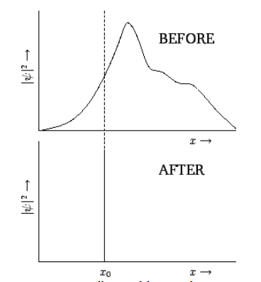
Consider an extended wavefunction, \(\psi(x,t)\). According to our usual interpretation, \(|\psi(x,t)|^{\,2}\) is proportional to the probability density of a measurement of the particle’s position yielding the value \(x\) at time \(t\). If the wavefunction is extended then there is a wide range of likely values that this measurement could give. Suppose that we make such a measurement, and obtain the value \(x_0\). We now know that the particle is located at \(x=x_0\). If we make another measurement immediately after the first one then common sense tells us that we must obtain the same value, \(x_0\), because the particle cannot have shifted position appreciably in an infinitesimal time interval. Thus, immediately after the first measurement, a measurement of the particle’s position is certain to give the value \(x_0\), and has no chance of giving any other value. This implies that the wavefunction must have collapsed to some sort of “spike” function located at \(x=x_0\). This is illustrated in Figure [coll]. Of course, as soon as the wavefunction has collapsed, it starts to expand again, as discussed in Section 1.13. Thus, the second measurement must be made reasonably quickly after the first, in order to guarantee that the same result will be obtained.

Figure 9: Collapse of the wavefunction upon measurement of ![]() .
.
The previous discussion illustrates an important point in quantum mechanics. Namely, that the wavefunction of a particle changes discontinuously (in time) whenever a measurement is made. We conclude that there are two types of time evolution of the wavefunction in quantum mechanics. First, there is a smooth evolution that is governed by Schrödinger’s equation. This evolution takes place between measurements. Second, there is a discontinuous evolution that takes place each time a measurement is made.
Contributors and Attributions
Richard Fitzpatrick (Professor of Physics, The University of Texas at Austin)
\( \newcommand {\ltapp} {\stackrel {_{\normalsize<}}{_{\normalsize \sim}}}\) \(\newcommand {\gtapp} {\stackrel {_{\normalsize>}}{_{\normalsize \sim}}}\) \(\newcommand {\btau}{\mbox{\boldmath$\tau$}}\) \(\newcommand {\bmu}{\mbox{\boldmath$\mu$}}\) \(\newcommand {\bsigma}{\mbox{\boldmath$\sigma$}}\) \(\newcommand {\bOmega}{\mbox{\boldmath$\Omega$}}\) \(\newcommand {\bomega}{\mbox{\boldmath$\omega$}}\) \(\newcommand {\bepsilon}{\mbox{\boldmath$\epsilon$}}\)

