4.2: Square Potential Barrier

Infinite Potential Well

Consider a particle of mass \(m\) and energy \(E\) moving in the following simple potential:

\[V(x) = \left\{\begin{array}{lcl} 0&\mbox{\hspace{1cm}}&\mbox{for $0\leq x\leq a$}\\[4pt] \infty&&\mbox{otherwise} \end{array}\right.. \nonumber \]

It follows from Equation \ref{e5.2} that if \(d^2\psi/d x^2\) (and, hence, \(\psi\)) is to remain finite then \(\psi\) must go to zero in regions where the potential is infinite. Hence, \(\psi=0\) in the regions \(x\leq 0\) and \(x\geq a\). Evidently, the problem is equivalent to that of a particle trapped in a one-dimensional box of length \(a\). The boundary conditions on \(\psi\) in the region \(0<x<a\) are

\[ \psi(0) = \psi(a) = 0. \label{e5.4} \]

Furthermore, it follows from Equation \ref{e5.2} that \(\psi\) satisfies

\[ \frac{d^2 \psi}{d x^2} = - k^2\,\psi \label{e5.5} \]

in this region, where

\[ k^2 = \frac{2\,m\,E}{\hbar^2}. \label{e5.6} \]

Here, we are assuming that \(E>0\). It is easily demonstrated that there are no solutions with \(E<0\) which are capable of satisfying the boundary conditions \ref{e5.4}.

The solution to Equation \ref{e5.5}, subject to the boundary conditions \ref{e5.4}, is

\[\psi_n(x) = A_n\,\sin(k_n\,x), \nonumber \]

where the \(A_n\) are arbitrary (real) constants, and

\[ k_n = \frac{n\,\pi}{a}, \label{e5.8} \]

for \(n=1,2,3,\cdots\). Now, it can be seen from Equations \ref{e5.6} and \ref{e5.8} that the energy \(E\) is only allowed to take certain discrete values: that is,

\[ E_n = \frac{n^2\,\pi^2\,\hbar^2}{2\,m\,a^2}. \label{eenergy} \]

In other words, the eigenvalues of the energy operator are discrete. This is a general feature of bounded solutions: that is, solutions for which \(|\psi|\rightarrow 0\) as \(|x|\rightarrow\infty\). According to the discussion in Section [sstat], we expect the stationary eigenfunctions \(\psi_n(x)\) to satisfy the orthonormality constraint

\[\int_0^a \psi_n(x)\,\psi_m(x)\,dx = \delta_{nm}. \nonumber \]

It is easily demonstrated that this is the case, provided \(A_n = \sqrt{2/a}\). Hence,

\[ \psi_n(x) = \sqrt{\frac{2}{a}}\,\sin\left(n\,\pi\,\frac{x}{a}\right) \label{e5.11} \]

for \(n=1,2,3,\cdots\).

Finally, again from Section [sstat], the general time-dependent solution can be written as a linear superposition of stationary solutions:

\[\psi(x,t) = \sum_{n=0,\infty} c_n\,\psi_n(x)\,\rm e^{-{\rm i}\,E_n\,t/\hbar}, \nonumber \]

where

\[ c_n = \int_0^a\psi_n(x)\,\psi(x,0)\,dx. \label{e5.13} \]

Square Potential Barrier

Consider a particle of mass \(m\) and energy \(E>0\) interacting with the simple square potential barrier

\[V(x) = \left\{\begin{array}{lcl} V_0&\mbox{\hspace{1cm}}&\mbox{for $0\leq x\leq a$}\\[4pt] 0&&\mbox{otherwise} \end{array} \right., \nonumber \]

where \(V_0>0\). In the regions to the left and to the right of the barrier, \(\psi(x)\) satisfies

\[ \frac{d^2 \psi}{d x^2} = - k^2\,\psi, \label{e5.15} \]

where \(k\) is given by Equation \ref{e5.6}.

Let us adopt the following solution of the previous equation to the left of the barrier (i.e., \(x<0\)):

\[\psi(x) = \rm e^{\,{\rm i}\,k\,x} + R\,\rm e^{-{\rm i}\,k\,x}. \nonumber \]

This solution consists of a plane-wave of unit amplitude traveling to the right [because the time-dependent wavefunction is multiplied by \(\exp(-{\rm i}\,\omega\,t)\), where \(\omega=E/\hbar>0\)], and a plane wave of complex amplitude \(R\) traveling to the left. We interpret the first plane wave as an incoming particle (or, rather, a stream of incoming particles), and the second as a particle (or stream of particles) reflected by the potential barrier. Hence, \(|R|^2\) is the probability of reflection. This can be seen by calculating the probability current \ref{eprobc} in the region \(x<0\), which takes the form

\[j_l=v\,(1-|R|^2), \nonumber \]

where \(v = p/m=\hbar\,k/m\) is the classical particle velocity.

Let us adopt the following solution to Equation \ref{e5.15} to the right of the barrier (i.e. \(x>a\)):

\[\psi(x) = T\,\rm e^{\,{\rm i}\,k\,x}. \nonumber \]

This solution consists of a plane-wave of complex amplitude \(T\) traveling to the right. We interpret this as a particle (or stream of particles) transmitted through the barrier. Hence, \(|T|^2\) is the probability of transmission. The probability current in the region \(x>a\) takes the form

\[j_r = v\, |T|^2. \nonumber \]

Now, according to Equation \ref{ediffp}, in a stationary state (i.e., \(\partial |\psi|^2/\partial t = 0\)), the probability current is a spatial constant (i.e., \(\partial j/\partial x = 0\)). Hence, we must have \(j_l=j_r\), or

\[ |R|^2 + |T|^2 = 1. \label{e5.20} \]

In other words, the probabilities of reflection and transmission sum to unity, as must be the case, because reflection and transmission are the only possible outcomes for a particle incident on the barrier.

Inside the barrier (i.e., \(0\leq x \leq a\)), \(\psi(x)\) satisfies

\[ \frac{d^2 \psi}{d x^2} = - q^2\,\psi, \label{e5.21} \]

where

\[q^2 = \frac{2\,m\,(E-V_0)}{\hbar^2}. \nonumber \]

Let us, first of all, consider the case where \(E> V_0\). In this case, the general solution to Equation \ref{e5.21} inside the barrier takes the form

\[\psi(x) = A\,\rm e^{\,{\rm i}\,q\,x} +B\,\rm e^{-{\rm i}\,q\,x}, \nonumber \]

where \(q=\sqrt{2\,m\,(E-V_0)/\hbar^2}\).

Now, the boundary conditions at the edges of the barrier (i.e., at \(x=0\) and \(x=a\)) are that \(\psi\) and \(d\psi/d x\) are both continuous. These boundary conditions ensure that the probability current \ref{eprobc} remains finite and continuous across the edges of the boundary, as must be the case if it is to be a spatial constant.

Continuity of \(\psi\) and \(d\psi/d x\) at the left edge of the barrier (i.e., \(x=0\)) yields

\[\begin{align} 1 + R &= A+B,\\[4pt] k\,(1-R) &= q\,(A-B).\end{align} \nonumber \]

Likewise, continuity of \(\psi\) and \(d\psi/d x\) at the right edge of the barrier (i.e., \(x=a\)) gives

\[\begin{align} A\, \rm e^{\,{\rm i}\,q\,a}+ B \,\rm e^{-{\rm i}\,q\,a} &= T\,\rm e^{\,{\rm i}\,k\,a},\\[4pt] q\left(A\,\rm e^{\,{\rm i}\,q\,a} -B \,\rm e^{-{\rm i}\,q\,a}\right) &=k\,T\,\rm e^{\,{\rm i}\,k\,a}.\end{align} \nonumber \]

After considerable algebra, the previous four equations yield

\[ |R|^2 = \frac{(k^2-q^2)^2\,\sin^2(q\,a)}{4\,k^2\,q^2 + (k^2-q^2)^2\,\sin^2(q\,a)}, \label{e5.28} \]

and

\[ |T|^2 = \frac{4\,k^2\,q^2}{4\,k^2\,q^2 + (k^2-q^2)^2\,\sin^2(q\,a)}. \label{e5.29} \]

Note that the previous two expression satisfy the constraint \ref{e5.20}.

It is instructive to compare the quantum mechanical probabilities of reflection and transmission—\ref{e5.28} and \ref{e5.29}, respectively—with those derived from classical physics. Now, according to classical physics, if a particle of energy \(E\) is incident on a potential barrier of height \(V_0<E\) then the particle slows down as it passes through the barrier, but is otherwise unaffected. In other words, the classical probability of reflection is zero, and the classical probability of transmission is unity.

The reflection and transmission probabilities obtained from Equations \ref{e5.28} and \ref{e5.29}, respectively, are plotted in Figures [fb1] and [fb2]. It can be seen, from Figure [fb1], that the classical result, \(|R|^2=0\) and \(|T|^2=1\), is obtained in the limit where the height of the barrier is relatively small (i.e., \(V_0\ll E\)). However, when \(V_0\) is of order \(E\), there is a substantial probability that the incident particle will be reflected by the barrier. According to classical physics, reflection is impossible when \(V_0 < E\).

It can also be seen, from Figure [fb2], that at certain barrier widths the probability of reflection goes to zero. It turns out that this is true irrespective of the energy of the incident particle. It is evident, from Equation \ref{e5.28}, that these special barrier widths correspond to

\[q\,a = n\,\pi, \nonumber \]

where \(n=1,2,3,\cdots\). In other words, the special barriers widths are integer multiples of half the de Broglie wavelength of the particle inside the barrier. There is no reflection at the special barrier widths because, at these widths, the backward traveling wave reflected from the left edge of the barrier interferes destructively with the similar wave reflected from the right edge of the barrier to give zero net reflected wave.

Let us, now, consider the case \(E< V_0\). In this case, the general solution to Equation \ref{e5.21} inside the barrier takes the form

\[\psi(x) = A\,\rm e^{\,q\,x} + B\,\rm e^{-q\,x}, \nonumber \]

where \(q=\sqrt{2\,m\,(V_0-E)/\hbar^2}\). Continuity of \(\psi\) and \(d \psi/d x\) at the left edge of the barrier (i.e., \(x=0\)) yields

\[\begin{align} 1 + R &=A+B,\\[4pt] {\rm i}\,k\,(1-R) &= q\,(A-B).\end{align} \nonumber \]

Likewise, continuity of \(\psi\) and \(d\psi/d x\) at the right edge of the barrier (i.e., \(x=a\)) gives

\[\begin{align} A\, \rm e^{\,q\,a}+ B \,\rm e^{-q\,a} &= T\,\rm e^{\,{\rm i}\,k\,a},\\[4pt] q\left(A\, \rm e^{\,q\,a}-B \,\rm e^{-q\,a}\right) &= {\rm i}\,k\,T\,\rm e^{\,{\rm i}\,k\,a}.\end{align} \nonumber \]

After considerable algebra, the previous four equations yield

\[ |R|^2 = \frac{(k^2+q^2)^2\,\sinh^2(q\,a)}{4\,k^2\,q^2 + (k^2+q^2)^2\,\sinh^2(q\,a)}, \label{e5.36} \]

and

\[ |T|^2 = \frac{4\,k^2\,q^2}{4\,k^2\,q^2 + (k^2+q^2)^2\,\sinh^2(q\,a)}. \label{e5.37} \]

These expressions can also be obtained from Equations \ref{e5.28} and \ref{e5.29} by making the substitution \(q\rightarrow -{\rm i}\,q\). Note that Equations \ref{e5.36} and \ref{e5.37} satisfy the constraint \ref{e5.20}.

It is again instructive to compare the quantum mechanical probabilities of reflection and trans/-mission—\ref{e5.36} and \ref{e5.37}, respectively—with those derived from classical physics. Now, according to classical physics, if a particle of energy \(E\) is incident on a potential barrier of height \(V_0>E\) then the particle is reflected. In other words, the classical probability of reflection is unity, and the classical probability of transmission is zero.

The reflection and transmission probabilities obtained from Equations \ref{e5.36} and \ref{e5.37}, respectively, are plotted in Figures [fb3] and [fb4]. It can be seen, from Figure [fb3], that the classical result, \(|R|^2=1\) and \(|T|^2=0\), is obtained for relatively thin barriers (i.e., \(q\,a\sim 1\)) in the limit where the height of the barrier is relatively large (i.e., \(V_0\gg E\)). However, when \(V_0\) is of order \(E\), there is a substantial probability that the incident particle will be transmitted by the barrier. According to classical physics, transmission is impossible when \(V_0 > E\).

It can also be seen, from Figure [fb4], that the transmission probability decays exponentially as the width of the barrier increases. Nevertheless, even for very wide barriers (i.e., \(q\,a\gg 1\)), there is a small but finite probability that a particle incident on the barrier will be transmitted. This phenomenon, which is inexplicable within the context of classical physics, is called tunneling.

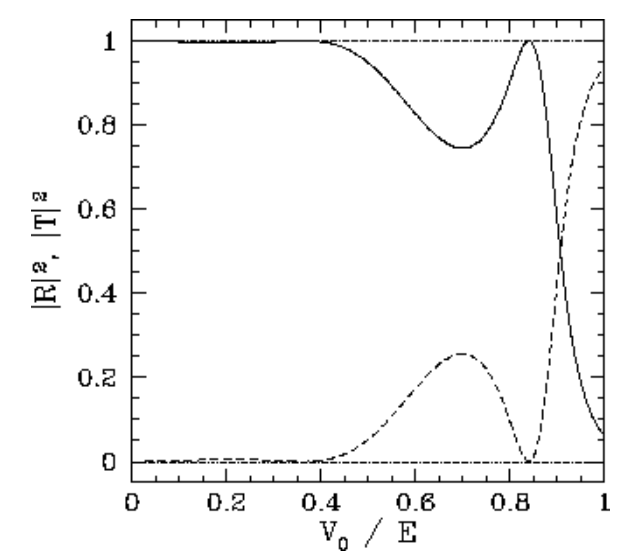
Figure 10: Transmission (solid-curve) and reflection (dashed-curve) probabilities for a square potential barrier of width \(a=1.25 \lambda\), where \(\lambda\) the free-space de Broglie wavelength, as a function of the ratio of the height of the barrier, \(V_{0}\), to the energy, \(E\), of the incident particle.

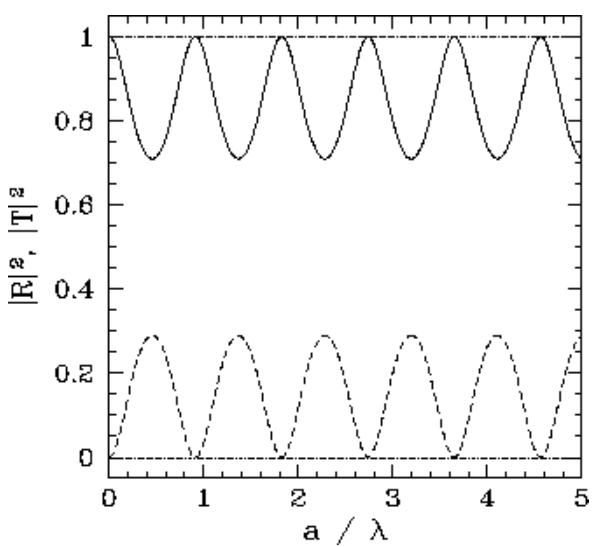
Figure 11: Transmission (solid-curve) and reflection (dashed-curve) probabilities for a particle of energy incident on a square potential barrier of height \(V_{0}=0.75 E\), as a function of the ratio of the width of the barrier, \(a\), to the free-space de Broglie wavelength, \(\lambda\)

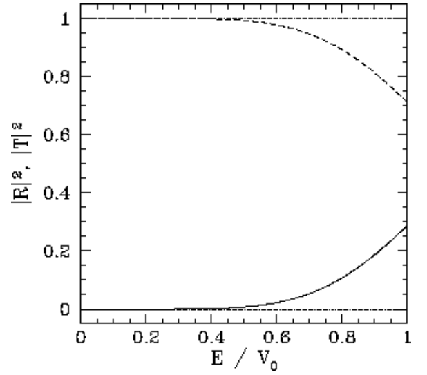
Figure 12: Transmission (solid-curve) and reflection (dashed-curve) probabilities for a square potential barrier of width \(a=0.5 \lambda \text { , where } \lambda \text { is }\)the free-space de Broglie wavelength, as a function of the ratio of the energy, , of the incoming particle to the height, \(V_{0}\),of the barrier.

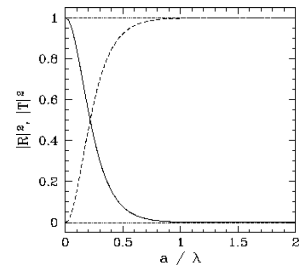
Figure 13: Transmission (solid-curve) and reflection (dashed-curve) probabilities for a particle of energy incident on a square potential barrier of height \(V_{0}=(4 / 3) E\), as a function of the ratio of the width of the barrier, , to the free-space de Broglie wavelength, \(\lambda\)