4.6: The Hydrogen Atom

Factoring Out the Center of Mass Motion

The hydrogen atom consists of two particles, the proton and the electron, interacting via the Coulomb potential $V(\vec{r_1}-\vec{r_2})=e^2/r$, where as usual $r=|\vec{r_1}-\vec{r_2}|$. Writing the masses of the two particles as $m_1, m_2$ Schrödinger’s equation for the atom is: $$\left( -\frac{\hbar^2}{2m_1}\vec{\nabla_1}^2-\frac{\hbar^2}{2m_2}\vec{\nabla_2}^2-\frac{e^2}{r}\right) \psi(\vec{r_1},\vec{r_2})=E\psi(\vec{r_1},\vec{r_2}). \label{4.6.1}$$

But $\vec{r_1},  \vec{r_2}$ are not the most natural position variables for describing this system: since the potential depends only on the relative position, a better choice is $\vec{r}, \vec{R}$ defined by: $$\vec{r}=\vec{r_1}-\vec{r_2},\;\; \vec{R}=\frac{m_1\vec{r_1}+m_2\vec{r_2}}{m_1+m_2} \label{4.6.2}$$

so $\vec{R}$ is the center of mass of the system. It is convenient at the same time to denote the total mass by $M=m_1+m_2$, and the reduced mass by $m=\frac{m_1m_2}{m_1+m_2}$.

Transforming in straightforward fashion to the variables $\vec{r},  \vec{R}$ Schrödinger’s equation becomes $$\left(-\frac{\hbar^2}{2M}\vec{\nabla_R}^2-\frac{\hbar^2}{2m}\vec{\nabla_r}^2-\frac{e^2}{r}\right)\psi(\vec{R}, \vec{r})=E\psi(\vec{R}, \vec{r}). \label{4.6.3}$$

Writing the wave function $$\psi(\vec{R}, \vec{r})=\Psi(\vec{R})\psi(\vec{r}) \label{4.6.4}$$

we can split the equation into two: $$\begin{matrix} \left( -\frac{\hbar^2}{2M}\vec{\nabla_R}^2\right) \Psi(\vec{R})=E_R\Psi(\vec{R}) \\ \left( -\frac{\hbar^2}{2m}\vec{\nabla_r}^2+V(\vec{r})\right) \psi(\vec{r})=Er\psi(\vec{r}) \end{matrix}\label{4.6.5}$$

and the total system energy is $E=E_R+E_r$. Note that the motion of the center of mass is (of course) just that of a free particle, having a trivial plane wave solution. From now on, we shall only be concerned with the relative motion of the particles. Since the proton is far heavier than the electron, we will almost always ignore the difference between the electron mass and the reduced mass, but it should be noted that the difference is easily detectable spectroscopically: for example, the lines shift if the proton is replaced by a deuteron (heavy hydrogen).

We’re ready to write Schrödinger’s equation for the hydrogen atom, dropping the r suffixes in the second equation above, and writing out $\vec{\nabla}^2$ explicitly in spherical coordinates:

$$\begin{matrix} -\frac{\hbar^2}{2m}\left( \frac{1}{r^2}\frac{\partial}{\partial r}\left( r^2\frac{\partial\psi}{\partial r}\right) +\frac{1}{r^2 \sin\theta}\frac{\partial}{\partial\theta}\left( \sin\theta\frac{\partial\psi}{\partial\theta}\right) +\frac{1}{r^2\sin^2\theta}\frac{\partial^2\psi}{\partial\varphi^2}\right) -\frac{e^2}{r}\psi \\ =E\psi. \end{matrix} \label{4.6.6}$$

Factoring Out the Angular Dependence: the Radial Equation - $R(r)$

Since the potential is spherically symmetric, the Hamiltonian $H$ commutes with the angular momentum operators $L^2$, $L_z$ so we can construct a common set of eigenkets of the three operators $H$, $L^2$, $L_z$. The angular dependence of these eigenkets is therefore that of the $Y^m_l$’s, so the solutions must be of the form

$$\psi_{Elm}(r,\theta,\phi)=R_{Elm}(r)Y^m_l(\theta,\phi). \label{4.6.7}$$

Now, notice that in the Schrödinger equation above, the angular part of $\vec{\nabla}^2$ is exactly the differential operator $L^2/2mr^2$, so operating on $\psi_{Elm}(r,\theta,\phi)=R_{Elm}(r)Y^m_l(\theta,\phi)$ it will give $\hbar^2l(l+1)/2mr^2$. The spherical harmonic $Y^m_l$ can then be cancelled from the two sides of the equation leaving:

$$\begin{matrix} -\dfrac{\hbar^2}{2m}\left( \dfrac{1}{r^2}\dfrac{d}{dr}(r^2\dfrac{d}{dr})-\dfrac{l(l+1)}{r^2}\right) R_{El}(r)-\dfrac{e^2}{r}R_{El}(r) \\ =ER_{El}(r) \end{matrix} \label{4.6.8}$$

it now being apparent that $R(r)$ cannot depend on $m$.

The radial derivatives simplify if one factors out $1/r$ from the function $R$, writing

$$R_{El}(r)=\dfrac{u(r)}{r} \label{4.6.9}$$

and temporarily suppressing the $E$ and $l$ to reduce clutter.

The equation becomes:

$$-\dfrac{\hbar^2}{2m}\left( \dfrac{d^2}{dr^2}-\dfrac{l(l+1)}{r^2}\right) u(r)-\dfrac{e^2}{r}u(r)=Eu(r). \label{4.6.10}$$

Rearranging,

$$-\dfrac{\hbar^2}{2m}\dfrac{d^2u(r)}{dr^2}+\left( \dfrac{\hbar^2}{2m}\dfrac{l(l+1)}{r^2}-\dfrac{e^2}{r}\right) u(r)=Eu(r). \label{4.6.11A}$$

Note that this is the same as the Schrödinger equation for a particle in one dimension, restricted to $r>0$, in a potential (for $l\neq 0$ ) going to positive infinity at the origin, then negative and going to zero at large distances, so it always has a minimum for some positive $r$.

We are interested in bound states of the proton-electron system, so $E$ will be a negative quantity. At large separations, the wave equation simplifies to

$$-\dfrac{\hbar^2}{2m}\dfrac{d^2u(r)}{dr^2}\cong E u(r) (for\; large\; r) \label{4.6.11B}$$

having approximate solutions $e^{\kappa r}$, $e^{-\kappa r}$ where $\kappa =\sqrt{-2mE/\hbar^2}$. The bound states we are looking for, of course, have exponentially decreasing wave functions at large distances.

Going to a Dimensionless Variable

To further simplify the equation, we introduce the dimensionless variable $$\rho=\kappa r,\;\; \kappa =\sqrt{-2mE/\hbar^2} \label{4.6.12}$$

giving $$\frac{d^2u(\rho)}{d\rho^2}=\left( 1-\frac{2\nu}{\rho}+\frac{l(l+1)}{\rho^2}\right) u(\rho) \label{4.6.13}$$

where (for reasons which will become apparent shortly) we have introduced $\nu$ defined by $$2\nu=e^2\kappa /E. \label{4.6.14}$$

Notice that in transforming from $r$ to the dimensionless variable $\rho$ the scaling factor $\kappa$ depends on energy, so will be different for different energy bound states!

Consider now the behavior of the wave function near the origin. The dominant term for sufficiently small $\rho$ is the centrifugal one, so $$\frac{d^2u(\rho)}{d\rho^2}\cong \frac{l(l+1)}{\rho^2}u(\rho) \label{4.6.15}$$

for which the solutions are $u(\rho)\sim \rho^{-l}$, $u(\rho)\sim \rho^{l+1}$. Since the wave function cannot be singular, we choose the second.

We have established that the wave function decays as $e^{-\kappa r}=e^{-\rho}$ at large distances, and goes as $\rho^{l+1}$ close to the origin. Factoring out these two asymptotic behaviors, define $w(\rho)$ by $$u(\rho)=e^{-\rho}\rho^{l+1}w(\rho). \label{4.6.16}$$

It is straightforward (if tedious) to establish that $w(\rho)$ satisfies the differential equation: $$\rho\frac{d^2w(\rho)}{d\rho^2}+2(l+1-\rho)\frac{dw(\rho)}{d\rho}+2(\nu-(l+1))w(\rho)=0. \label{4.6.17}$$

Putting in a trial series solution $w(\rho)=\sum_{k=0}^{\infty}w_k\rho^k$ gives a recurrence relation between successive coefficients: $$\frac{w_{k+1}}{w_k}=\frac{2(k+l+1-\nu)}{(k+1)(k+2(l+1))}. \label{4.6.18}$$

For large values of $k$, $w_{k+1}/w_k\to 2/k$, so $w_k\sim 2^k/k!$ and therefore $w(\rho)\sim e^2\rho$. This means we have found the diverging radial wavefunction $u(\rho)\sim e^{\rho}$, which is in fact the correct behavior for general values of the energy.

To find the bound states, we must choose energies such that the series is not an infinite one. As long as the series stops somewhere, the exponential decrease will eventually take over, and yield a finite (bound state) wave function. Just as for the simple harmonic oscillator, this can only happen if for some $k, w_{k+1}=0$. Inspecting the ratio $w_{k+1}/w_k$, evidently the condition for a bound state is that $$\nu=n,\;\; an\; integer \label{4.6.19}$$

in which case the series for $w(\rho)$ terminates at $k=n-l-1$. From now on, since we know that for the functions we’re interested in $\nu$ is an integer, we replace $\nu$ by $n$.

To find the energies of these bound states, recall $2n=2\nu=e^2\kappa /E$ and $\kappa =\sqrt{-2mE/\hbar^2}$, so $$4n^2=\frac{e^4\kappa_n^2}{E_n^2}=-\frac{e^4}{E_n^2}\frac{2mE_n}{\hbar^2}, \label{4.6.20}$$

so $$E_n=-\frac{me^4}{2\hbar^2}\frac{1}{n^2}=-\frac{13.6}{n^2} ev = -\frac{1}{n^2} Rydberg. \label{4.6.21}$$

(This defines the Rydberg, a popular unit of energy in atomic physics.)

Remarkably, this is the very same series of bound state energies found by Bohr from his model! Of course, this had better be the case, since the series of energies Bohr found correctly accounted for the spectral lines emitted by hot hydrogen atoms. Notice, though, that there are some important differences with the Bohr model: the energy here is determined entirely by $n$, called the principal quantum number, but, in contrast to Bohr’s model, $n$ is not the angular momentum. The true ground state of the hydrogen atom, $n=1$, has zero angular momentum: since $n=k+l+1$, $n=1$ means both $l=0$ and $k=0$. The ground state wave function is therefore spherically symmetric, and the function $w(\rho)=w_0$ is just a constant. Hence $u(\rho)=\rho e^{-\rho}w_0$ and the actual radial wave function is this divided by $r$, and of course suitably normalized.

To write the wave function in terms of $r$, we need to find $\kappa$. Putting together $\rho=\kappa_n r$, $\kappa_n=\sqrt{-2mE_n/\hbar^2}$ and $E_n=-\frac{me^4}{2\hbar^2}\frac{1}{n^2}$, $$\kappa_n=\sqrt{2m\frac{me^4}{2\hbar^2}\frac{1}{n^2}}/\hbar=\frac{me^2}{\hbar^2n}=\frac{1}{a_0n}, \label{4.6.22}$$

where the length $$a_0=\frac{\hbar^2}{me^2}=0.529\times 10^{-10}m. \label{4.6.23}$$

is called the Bohr radius: it is in fact the radius of the lowest orbit in Bohr’s model.

Exercise: check this last statement.

It is worth noting at this point that the energy levels can be written in terms of the Bohr radius $a_0$: $$E_n=-\frac{e^2}{2a_0}\frac{1}{n^2}. \label{4.6.24}$$

(This is actually obvious: remember that the energies $E_n$ are identical to those in the Bohr model, in which the radius of the $n^{th}$ orbit is $n^2a_0$, so the electrostatic potential energy is $-e^2/na_0$, etc.)

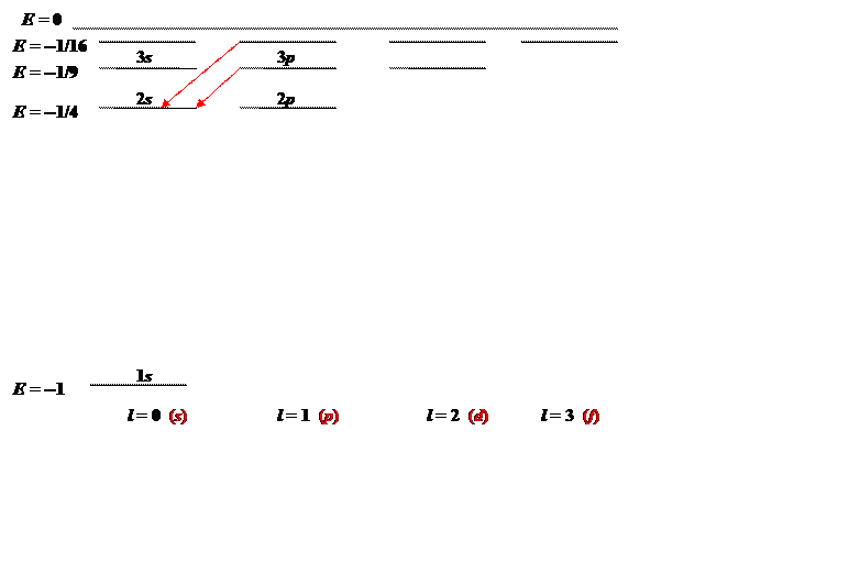
Moving on to the excited states: for $n=2$, we have a choice: either the radial function $w(\rho)$ can have one term, as before, but now the angular momentum $l=1$ (since $n=k+l+1$ ); or $w(\rho)$ can have two terms (so $k=1$ ), and $l=0$. Both options give the same energy, -0.25 Ry, since n is the same, and the energy only depends on $n$. In fact, there are four states at this energy, since $l=1$ has states with $m=1, m=0$ and $m=-1$, and $l=0$ has the one state $m=0$. (For the moment, we are not counting the extra factor of 2 from the two possible spin orientations of the electron.)

For $n=3$, there are 9 states altogether: gives one, $l=1$ gives 3 and $l=2$ gives 5 different $m$ values. In fact, for principal quantum number $n$ there are $n^2$ degenerate states. ( $n^2$ being the sum of the first $n$ odd integers.)

The states can be mapped out, energy vertically, angular momentum horizontally:

The energy $E=-1/n^2$, the levels are labeled $nl$, $n$ being the principal quantum number and the traditional notation for angular momentum $l$ is given at the bottom of the diagram. The two red vertical arrows are the first two transitions in the spectroscopic Balmer series, four lines of which gave Bohr the clue that led to his model. The corresponding series of transitions to the $1s$ ground state are in the ultraviolet, they are called the Lyman series.

Wave Functions for some Low-n States

From now on, we label the wave functions with the quantum numbers, $\psi_{nlm}(r,\theta,\phi)$, so the ground state is the spherically symmetric $\psi_{100}(r)$.

For this state $R(r)=u(r)/r$, where $u(\rho)=e^{-\rho}\rho^{l+1}w(\rho)=e^{-\rho}\rho w_0$, with $w_0$ a constant, and $\rho=\kappa_1 r=r/a_0$.

So, as a function of $r$, $\psi_{100}(r)=Ne^{-r/a_0}$ with $N$ an easily evaluated normalization constant:

$$\psi_{100}(r)=\left( \frac{1}{\pi a^3_0}\right)^{1/2}e^{-r/a_0}. \label{4.6.25}$$

For $n=2, l=1$ the function $w(\rho)$ is still a single term, a constant, but now $u(\rho)=e^{-\rho}\rho^{l+1}w(\rho)=e^{-\rho}\rho^2w_0$, and, for $n=2$,  $\rho=\kappa r=r/2a_0$, remembering the energy-dependence of $\kappa$.

Therefore $\psi_{210}(r,\theta,\phi)=N\left( \frac{r}{a_0}\right) e^{-r/2a_0}\cos\theta$. Again, evaluating the normalization constant is routine, yielding $$\psi_{210}(r,\theta,\phi)=\left( \frac{1}{32\pi a^3_0}\right)^{1/2}\left( \frac{r}{a_0}\right) e^{-r/2a_0}\cos\theta. \label{4.6.26}$$

The wave functions for the other $m$ -values, $\psi_{21\pm 1}(r,\theta,\phi)$, have the $\cos\theta$ in $\psi_{210}$ replaced by $\mp (1/\sqrt{2})\sin\theta e^{\pm i\phi}$ respectively (from the earlier discussion of the $Y^m_l$ ’s).

The other $n=2$ state has $l=0$, so from $n=k+l+1$, we have $k=1$ and the series for $w$ has two terms, $k=0$ and $k=1$, the ratio being

$$\frac{w_{k+1}}{w_k}=\frac{2(k+l+1-n)}{(k+1)(k+2(l+1))}=-1 \label{4.6.27}$$

for the relevant values: $k=0, l=0, n=2$. So $w_1=-w_0$, $w(\rho)=w_0(1-\rho)$. For $n=2$, $\rho=r/2a_0$, the normalized wave function is

$$\psi_{200}(r)=\left( \frac{1}{32\pi a^3_0}\right)^{1/2}\left( 2-\frac{r}{a_0}\right) e^{-r/2a_0}. \label{4.6.28}$$

Note that the zero angular momentum wave functions are nonzero and have nonzero slope at the origin. This means that the full three dimensional wave functions have a slope discontinuity there! But this is fine—the potential is infinite at the origin. (Actually, the proton is not a point charge, so really the kink will be smoothed out over a volume of the size of the proton—a very tiny effect.)

General Solution of the Radial Equation

In practice, the first few radial functions $w(\rho)$ can be constructed fairly easily using the method presented above, but it should be noted that the differential equation for $w(\rho)$ $$\rho \frac{d^2w(\rho)}{d\rho^2}+2(l+1-\rho)\frac{dw(\rho)}{d\rho}+2(n-(l+1))w(\rho)=0 \label{4.6.29}$$

is in fact Laplace’s equation, usually written $$\left( z\frac{d^2}{dz^2}+(k-1-z)\frac{d}{dz}+p\right) L^k_p(z)=0 \label{4.6.30}$$

where $k,p$ are integers, and $L^k_p(z)$ is a Laguerre polynomial (Messiah, page 482).

The two equations are the same if $z = 2\rho$, and the solution to the radial equation is therefore $$w_{nl}(\rho)=L^{2l+1}_{n-l-1}(2\rho). \label{4.6.31}$$

Quoting Messiah, the Laguerre polynomials $L^0_p(z)$, and the associated Laguerre polynomials $L^k_p(z)$ are given by:

$$\begin{matrix} L^0_p(z)=e^z\frac{d^p}{dz^p}e^{-z}z^p \\ L^k_p(z)=(-1)^k\frac{d^k}{dz^k}L^0_{p+k}(z). \end{matrix} \label{4.6.32}$$

(These representations can be found neatly by solving Laplace’s equation using – surprise – a Laplace transform. See Merzbacher for details.) The polynomials satisfy the orthonormality relations (with the mathematicians’ normalization convention)

$$\int^{\infty}_{0}e^{-z}z^k L^k_p L^k_qdz=\frac{[(p+k)!]^3}{p!}\delta_{pq}. \label{4.6.33}$$

But what do they look like? The function $e^{-z}z^p$ is zero at the origin (apart from the trivial case $p=0$ ) and zero at infinity, always positive and having nonzero slope except at its maximum value, $z=p$. The $p$ derivatives bring in $p$ separated zeroes, easily checked by sketching the curves generated by successive differentiation. Therefore, $L^0_p(z)$, a polynomial of degree $p$, has $p$ real positive zeroes, and value at the origin $L^0_p(0)=p!$, since the only nonzero term at $z=0$ is that generated by all $p$ differential operators acting on $z^p$.

The associated Laguerre polynomial $L^k_p(z)$ is generated by differentiating $L^0_{p+k}(z)$  $k$ times. Now $L^0_{p+k}(z)$ has $p+k$ real positive zeroes, differentiating it gives a polynomial one degree lower, with zeroes which must be one in each interval between the zeroes of $L^0_{p+k}(z)$. This argument remains valid for successive differentiations, so $L^k_p(z)$ must have $p$ real separate zeroes.

Putting all this together, and translating back from $\rho$ to $r$, the radial solutions are:

$$R_{nl}(r)=Ne^{-r/na_0}(\frac{r}{na_0})^l L^{2l+1}_{n-l-1}(\frac{2r}{na_0}) \label{4.6.34}$$

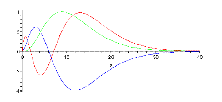
with $N$ the normalization constant. Griffiths (page 141) gives more details, including the normalization constants worked out. We used those to plot the $n=3$ states—plotting here the functions $u(r)=rR(r)$, since the normalization is $4\pi \int^{\infty}_{0}|u(r)|^2dr=1, u(r)$ gives a better idea of at what distance from the proton the electron is most likely to be found.

Here are the three $n=3$ radial wave functions:

The number of nodes, the radial quantum number, is $3-l-1$. (Note: The relative normalizations are correct here, but not the overall normalization.)

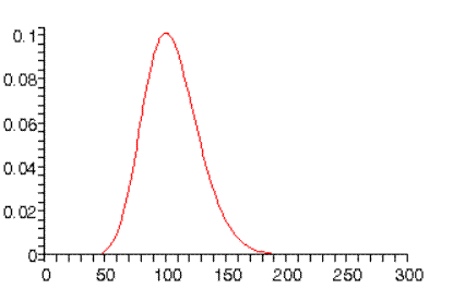
For higher $n$ values, the wave functions become reminiscent of classical mechanics. for example, for $n=10$, the highest angular momentum state probability distribution peaks at $r=100a_0$, the Bohr orbit radius:

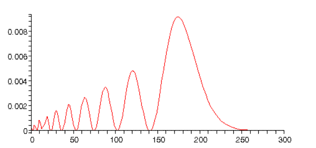
whereas for $n=10, l=0$, we find:

Notice this peaks just below twice the Bohr radius. This can be understood from classical mechanics: for an inverse square force law, elliptical orbits with the same semimajor axis have the same energy. The $l=n-1$ orbit is a circle, the $l=0$ orbit is a long thin ellipse (one end close to the proton), so it extends almost twice as far from the origin as the circle. Furthermore, the orbiting electron will spend longer at the far distance, since it will be moving very slowly. (Note: the normalizations in the above graphs are only approximate.)