5.2: Solution

Figure 5.1: The change in the wave function in region III, for the lowest state, as we increase the depth of the potential well. We have used a= 1 0− 1 0 m, and k 0 a= 2, 3, 4, 5, 6, 7, 8, 9 and 1 0.

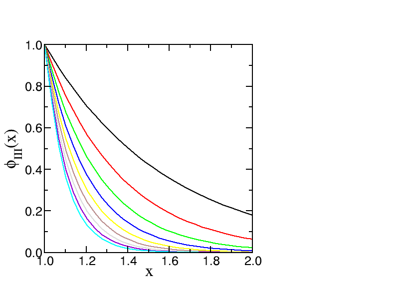
As stated before the continuity arguments for the derivative of the wave function do not apply for an infinite jump in the potential energy. This is easy to understand as we look at the behaviour of a low energy solution in one of the two outside regions (I or III). In this case the wave function can be approximated as

\[e ± k r\]

with \(k = 2 m ℏ^ 2 V 0\)

which decreases to zero faster and faster as V 0 becomes larger and larger. In the end the wave function can no longer penetrate the region of infinite potential energy. Continuity of the wave function now implies that ϕ( a)=ϕ(− a)= 0.

Defining

\[κ = \sqrt{ 2 m ℏ^ 2 E}\]

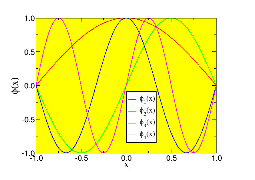
we find that there are two types of solutions that satisfy the boundary condition:

\[ϕ 2 n + 1 ( x ) = \cos ( κ 2 n + 1 x )\]

\[ ϕ 2 n ( x ) = \sin ( κ 2 n x ) .\]

Here

\[κ l = π l 2 a .\]

We thus have a series of eigenstates \(ϕ l( x), l= 1,⋯,∞). The energies are

\[E_l = ℏ^2 π^2 l 2 8 a^2.\]

Figure 5.2: A few wave functions of the infinite square well.

These wave functions are very good to illustrate the idea of normalisation. Let me look at the normalisation of the ground state (the lowest state), which is

\[ϕ 0 ( x ) = A 1 \cos π x 2 a\]

for − a< x< a, and 0 elsewhere.

We need to require

\∫ − ∞ ∞ | ϕ 0 ( x ) | 2 d x = 1 ,\]

where we need to consider the absolute value since A 1 can be complex. We only have to integrate from − a to a, since the rest of the integral is zero, and we have

\[∫ − ∞ ∞ | ϕ 0 ( x ) | 2 d x = | A | 2 ∫ − a a cos 2 π x 2 a d x = | A | 2 2 a π ∫ − π ∕ 2 π ∕ 2 cos 2 y d y = | A | 2 2 a π ∫ − π ∕ 2 π ∕ 2 1 2 ( 1 + cos 2 y ) d y = | A | 2 2 a π π . \]

Here we have changed variables from x to \(y=π x^2 a). We thus conclude that the choice

\[A = 1 2 a\]

leads to a normalised wave function.