
2.1: Bound States and Free States
- Page ID
- 34624

A curious feature of wavefunctions in infinite space is that they can have two distinct forms: (i) bound states that are localized to one region, and (ii) free states that extend over the whole space. Both kinds of states can co-exist in a single system. A simple model exhibiting this is the 1D finite square well. Consider the Hamiltonian
\[\hat{H} = \frac{\hat{p}^2}{2m} - U \,\Theta(a -|\hat{x}|),\]
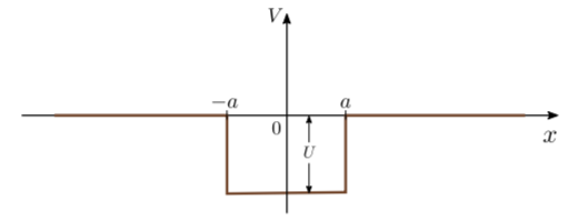
where \(\hat{x}\) and \(\hat{p}\) are 1D position and momentum operators, \(m\) is the particle mass, \(U\) and \(a\) are positive real parameters governing the potential function, and \(\Theta\) denotes the Heaviside step function (1 if the input is positive, and 0 otherwise). As shown below, the potential forms a well of depth \(U\) and width \(2a\). Outside the well, the potential is zero.
For such a Hamiltonian, the time-independent Schrödinger wave equation can be solved efficiently using a technique called the transfer matrix method. Here, we will describe a few key aspects of the calculation, bypassing most of the details. For a fuller discussion of the transfer matrix method, refer to Appendix B.
We begin by noting that obtaining solutions to the Schrödinger wave equation first requires specifying the boundary conditions at infinity. The choice of boundary conditions determines whether the solution we get is a bound state or free state.
For a bound state, we require the wavefunction to diminish exponentially as \(x \rightarrow \pm\infty\). In the exterior region (\(|x| > a\)), the Schrödinger wave equation reduces to
\[-\frac{\hbar^2}{2m}\,\frac{d^2\psi}{dx^2} = E \psi(x),\]
subject to the boundary conditions
\[\psi(x) \;\overset{x\rightarrow\pm\infty}{\sim} \; e^{\mp\kappa x}, \;\;\;\mathrm{Re}(\kappa) > 0.\]
Therefore, in the exterior region the bound state solutions take the form
\[\psi(x) = c_\pm\, e^{\mp\kappa x}, \;\;\mathrm{where}\;\, -\frac{\hbar^2\kappa^2}{2m} = E, \;\; c_\pm \in \mathbb{C}.\]
Given that \(E\) is real, it follows that \(\kappa\) is real, so \(E < 0\). Moreover, the variational principle implies that \(E \ge -U\), so bound state energies are restricted to the range \(-U \le E < 0\).
It is also possible to show that the bound state energies are discrete: the energy spacing decreases with \(a\), but so long as \(a\) is finite, the spacing is non-vanishing. Furthermore, the wavefunction for a bound state can always be normalized:
\[\int_{-\infty}^\infty |\psi(x)|^2\, dx\; =\; 1.\]
The normalization integral is finite since \(|\psi(x)|^2\) vanishes exponentially for \(x \rightarrow \pm \infty\). These properties follow from the analysis of the general class of “Sturm-Liouville-type” differential equations; for details, refer to textbooks such as Courant and Hilbert (1953).
For a free state, the situation is quite different. The wavefunction does not vanish exponentially at infinity, but takes the form
\[\psi(x) = \begin{cases} \alpha_-\, e^{ik x} + \beta_-\, e^{-ik x}, & \;\;\;x < -a\\ (\mathrm{something}) , & -a < x < a\\ \alpha_+\, e^{ik x} + \beta_+\, e^{-ik x} , & \;\;\,x > a.\end{cases}\]
Inside the potential well, \(\psi(x)\) varies in some complicated way; on the outside, it consists of superpositions of left-moving and right-moving plane waves with real wavenumber \(k\). The coefficients \(\alpha_\pm\) and \(\beta_\pm\) are not independent quantities, but are linked by a linear relation (see Appendix B). To satisfy Schrödinger’s equation, we must have
\[\frac{\hbar^2k^2}{2m} = E,\]
which implies that free states only occur for \(E \ge 0\). These solutions form a continuum: there are free states for every \(E \ge 0\). Since \(|\psi(x)|^2\) does not diminish at infinity, the integral \(\int_{-\infty}^\infty |\psi(x)|^2\, dx\) is divergent, so the wavefunctions have no finite normalization.
The following figure shows numerically-obtained results for a square well with \(U = 30\) and \(a=1\) (in units where \(\hbar = m =1\)). The energy spectrum is shown on the left side. There exist five bound states; their plots of \(|\psi|^2\) versus \(x\) are shown on the right side. These results were computed using the transfer matrix method described in Appendix B.

Many of the lessons drawn from the square well model can be generalized to more complicated potentials. In cases where the potential at infinity is \(V_{\textrm{ext}}\) rather than zero, free states occur for \(E \ge V_{\textrm{ext}}\) and bound states occur for \(\textrm{min}(V) < E < V_{\textrm{ext}}\).
There is an important proviso to bear in mind. If we vary the potential, the number of bound states can change: i.e., bound state solutions can either appear or disappear. A numerical example is given below, showing the bound state energies for the square well model with fixed \(a = 1\), as we vary the potential minimum \(-U\):
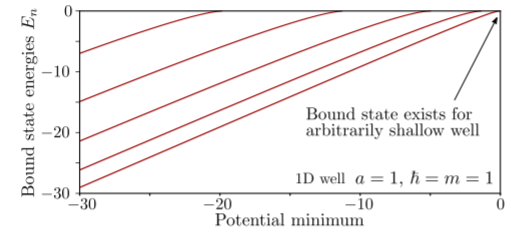
For \(U = 30\), there are five bound states, which disappear one by one as we make the potential well shallower. Note that one bound state survives in the limit \(U \rightarrow 0\). There is a theorem stating that any 1D attractive potential, no matter how weak, always supports at least one bound state. For details, see Exercise 2.6.1.
In 3D, it is possible for an attractive potential to be too weak to support a bound state. Intuitively, this happens when the zero-point energy of a prospective ground state exceeds the well depth. The figure below shows a numerical example, calculated for a uniform 3D spherically symmetric well (the \(l\)’s labeling the various curves are angular momentum quantum numbers). To learn more about this phenomenon, refer to Exercise 2.6.2.
