2.2: Quasi-Bound States and Resonances

For the 1D finite square well, there is a clear distinction between bound and free states. Certain potentials, however, can host a special class of states called “quasi-bound states”. Like a bound state, a quasi-bound state is localized in one region of space. However, it is an approximate eigenstate of the Hamiltonian that lies in the energy range of the free state continuum. As we shall see, quasi-bound states play an important important role in scattering experiments.

The figure below shows an example of a potential function that gives rise to quasi-bound states. In the exterior region, \(|x| > b\), the potential is zero. Between \(x = -b\) and \(x = b\), there is a “barrier” of positive potential \(V_b\). Embedded in the middle of this barrier, for \(|x| < a\), is a central well of depth \(U\), where \(0 < V_b - U < V_b\).

Figure \(\PageIndex{1}\)

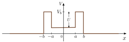
This potential is purely repulsive (\(V \ge 0\) everywhere), so there are no true bound states. The only exact eigenstates of the Hamiltonian are free states.

However, there is something intriguing about the central well. Consider an alternative scenario where the potential in the exterior region is \(V_b\) rather than \(0\); i.e., the potential function is a finite square well:

\[V_{\mathrm{alt}}(x) = \begin{cases}V_b - U, & |x| < a, \\ V_b, & \mathrm{otherwise}.\end{cases}\]

In this case, there would be one or more bound states, in the energy range \(V_b-U < E < V_b\). These bound states’ wavefunctions diminish exponentially away from the well, and are thus close to zero for \(|x| > b\). Since \(V(x)\) and \(V_{\mathrm{alt}}(x)\) differ only in the region \(|x| > b\), these wavefunctions ought to be approximate solutions to the Schrödinger wave equation for the original potential \(V(x)\), which does not support bound states! Such approximate solutions are called quasi-bound states.

Let us analyze the potential \(V(x)\) using the scattering experiment framework from the previous chapter. Consider an incident particle of energy \(E > 0\) whose wavefunction is

\[\psi_i(x) = \Psi_i \, e^{ik_i x}.\]

This produces a scattered wavefunction \(\psi_s(x)\) that is outgoing (as discussed in the previous chapter). In the exterior region, the scattered wavefunction takes the form

\[\psi_s(x) = \Psi_i \times \begin{cases}f_- \,e^{-ik_ix}, & x \le -b \\ f_+ \,e^{ik_ix}, & x \ge b.\end{cases}\]

The scattering amplitudes \(f_+\) and \(f_-\) can be found by solving the Schrödinger wave equation using the transfer matrix method (see Appendix B). The figure below shows numerical results obtained for \(U = 20,\,V_b = 30,\,a=1\), and \(b = 1.2\) or \(b = 1.4\), with \(\hbar = m = 1\).

Figure \(\PageIndex{2}\)

The vertical axis shows \(|1+f_+|^2\), which is called the “transmittance” and corresponds to the probability for the incident particle to pass through the potential. The horizontal axis is the particle energy \(E\). For \(E < V_b-U\), the transmittance approaches zero, and for \(E \gtrsim V_b\), the transmittance approaches unity, as expected. In the energy range \(V_b-U < E \lesssim V_b\), the transmittance forms a series of narrow peaks. For larger \(b\) (i.e., when the central well is more isolated from the exterior space), the peaks are narrower. At the top of the figure, we have also plotted the bound state energies for the square well potential \(V_{\mathrm{alt}}(x)\). These energies closely match the locations of the transmittance peaks!

Upon examining the total wavefunction \(\psi(x)\) at these special energies, we find other interesting features. The figure below plots \(|\psi(x)|^2\) versus \(x\) at the energies of the first three transmittance peaks, along with the corresponding bound state wavefunctions for the square well \(V_{\mathrm{alt}}\). At each transmittance peak, \(|\psi(x)|^2\) is much larger within the potential region, and its shape is very similar to a square well bound state.

Figure \(\PageIndex{3}\)

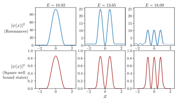
The enhancement of \(|\psi(x)|^2\) is called a resonance. It happens because of the existence of a quasi-bound state—an approximate energy eigenstate localized in the scattering region. When an incident particle enters the scattering region with the right energy, it spends a long time trapped in the quasi-bound state, before eventually escaping back to infinity.

This is analogous to the phenomenon of resonance in a classical harmonic oscillator. When a damped harmonic oscillator is subjected to an oscillatory driving force, it settles into a steady-state oscillatory motion at the driving frequency. If the driving frequency matches the oscillator’s natural frequency, the amplitude of the oscillation becomes large, and the system is said to be “resonant”. In the quantum mechanical context, the incident wavefunction plays the role of a driving force, the incident particle energy is like the driving frequency, and the energy of a quasi-bound state is like a natural frequency of oscillation.

Resonances play a critical role throughout experimental physics. Experiments are often conducted for the express purpose of locating and studying resonances. When a resonance peak is found, its location and shape can be used to deduce various features of the quasi-bound state, which in turn supplies important information about the underlying system.